Temporal Logic and Model Checking Model mathematical structure - PowerPoint PPT Presentation
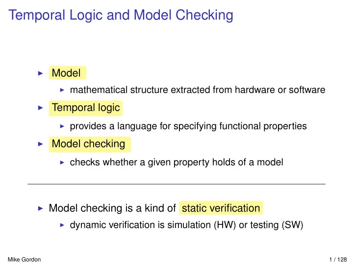
Temporal Logic and Model Checking Model mathematical structure extracted from hardware or software Temporal logic provides a language for specifying functional properties Model checking checks whether a given property holds
State satisfying NotAt11 unreachable from ( 0 , 0 , 0 , 0 ) Thread 1 Thread 2 0: IF LOCK=0 THEN LOCK:=1; 0: IF LOCK=0 THEN LOCK:=1; 1: X:=1; 1: X:=2; 2: IF LOCK=1 THEN LOCK:=0; 2: IF LOCK=1 THEN LOCK:=0; 3: 3: R JM1 ( pc 1 , 0 , 0 , x ) ( pc 1 , 1 , 1 , x ) R JM1 ( 0 , pc 2 , 0 , x ) ( 1 , pc 2 , 1 , x ) R JM1 ( 1 , pc 2 , lock , x ) ( 2 , pc 2 , lock , 1 ) R JM1 ( pc 1 , 1 , lock , x ) ( pc 1 , 2 , lock , 2 ) R JM1 ( 2 , pc 2 , 1 , x ) ( 3 , pc 2 , 0 , x ) R JM1 ( pc 1 , 2 , 1 , x ) ( pc 1 , 3 , 0 , x ) NotAt11 ( pc 1 , pc 2 , lock , x ) = ¬ (( pc 1 = 1 ) ∧ ( pc 2 = 1 )) ◮ ◮ Can only reach pc 1 = 1 ∧ pc 2 = 1 via: i.e. a step R JM1 ( 0 , 1 , 0 , x ) ( 1 , 1 , 1 , x ) R JM1 ( 0 , pc 2 , 0 , x ) ( 1 , pc 2 , 1 , x ) i.e. a step R JM1 ( 1 , 0 , 0 , x ) ( 1 , 1 , 1 , x ) R JM1 ( pc 1 , 0 , 0 , x ) ( pc 1 , 1 , 1 , x ) ◮ But: R JM1 ( pc 1 , pc 2 , lock , x ) ( pc ′ 1 , pc ′ 2 , lock ′ , x ′ ) ∧ pc ′ 1 = 0 ∧ pc ′ 2 = 1 ⇒ lock ′ = 1 ∧ R JM1 ( pc 1 , pc 2 , lock , x ) ( pc ′ 1 , pc ′ 2 , lock ′ , x ′ ) ∧ pc ′ 1 = 1 ∧ pc ′ 2 = 0 ⇒ lock ′ = 1 ◮ So can never reach ( 0 , 1 , 0 , x ) or ( 1 , 0 , 0 , x ) ◮ So can’t reach ( 1 , 1 , 1 , x ) , hence never ( pc 1 = 1 ) ∧ ( pc 2 = 1 ) ◮ Hence all states reachable from ( 0 , 0 , 0 , 0 ) satisfy NotAt11 Mike Gordon 16 / 128
Reachability ◮ R s s ′ means s ′ reachable from s in one step ◮ R n s s ′ means s ′ reachable from s in n steps R 0 s s ′ = ( s = s ′ ) R n + 1 s s ′ = ∃ s ′′ . R s s ′′ ∧ R n s ′′ s ′ ◮ R ∗ s s ′ means s ′ reachable from s in finite steps R ∗ s s ′ = ∃ n . R n s s ′ ◮ Note: R ∗ s s ′ ⇔ ∃ π n . Path R s π ∧ ( s ′ = π ( n )) ◮ The set of states reachable from s is { s ′ | R ∗ s s ′ } ◮ Verification problem: all states reachable from s satisfy p ◮ verify truth of ∀ s ′ . R ∗ s s ′ ⇒ p ( s ′ ) ◮ e.g. all states reachable from ( 0 , 0 , 0 , 0 ) satisfy NotAt11 JM1 ( 0 , 0 , 0 , 0 ) s ′ ⇒ NotAt11 ( s ′ ) ◮ i.e. ∀ s ′ . R ∗ Mike Gordon 17 / 128
Models and model checking ◮ Assume a model ( S , R ) ◮ Assume also a set S 0 ⊆ S of initial states ◮ Assume also a set AP of atomic properties ◮ allows different models to have same atomic properties ◮ Assume a labelling function L : S → P ( AP ) ◮ p ∈ L ( s ) means “ s labelled with p ” or “ p true of s ” ◮ previously properties were functions p : S → B ◮ now p ∈ AP is distinguished from λ s . p ∈ L ( s ) ◮ assume T , F ∈ AP with forall s : T ∈ L ( s ) and F / ∈ L ( s ) ◮ A Kripke structure is a tuple ( S , S 0 , R , L ) ◮ often the term “model” is used for a Kripke structure ◮ i.e. a model is ( S , S 0 , R , L ) rather than just ( S , R ) ◮ Model checking computes whether ( S , S 0 , R , L ) | = φ ◮ φ is a property expressed in a property language ◮ informally M | = φ means “wff φ is true in model M ” Mike Gordon 18 / 128
Minimal property language: φ is AG p where p ∈ AP ◮ Consider properties φ of form AG p where p ∈ AP ◮ “ AG ” stands for “Always Globally” ◮ from CTL (same meaning, more elaborately expressed) ◮ Assume M = ( S , S 0 , R , L ) ◮ Reachable states of M are { s ′ | ∃ s ∈ S 0 . R ∗ s s ′ } ◮ i.e. the set of states reachable from an initial state ◮ Define Reachable M = { s ′ | ∃ s ∈ S 0 . R ∗ s s ′ } ◮ M | = AG p means p true of all reachable states of M ◮ If M = ( S , S 0 , R , L ) then M | = φ formally defined by: = AG p ⇔ ∀ s ′ . s ′ ∈ Reachable M ⇒ p ∈ L ( s ′ ) M | Mike Gordon 19 / 128
Model checking M | = AG p = AG p ⇔ ∀ s ′ . s ′ ∈ Reachable M ⇒ p ∈ L ( s ′ ) ◮ M | ⇔ Reachable M ⊆ { s ′ | p ∈ L ( s ′ ) } checked by: ◮ first computing Reachable M ◮ then checking p true of all its members ◮ Let S abbreviate { s ′ | ∃ s ∈ S 0 . R ∗ s s ′ } (i.e. Reachable M ) ◮ Compute S iteratively: S = S 0 ∪ S 1 ∪ · · · ∪ S n ∪ · · · ◮ i.e. S = � ∞ n = 0 S n ◮ where: S 0 = S 0 (set of initial states) ◮ and inductively: S n + 1 = S n ∪ { s ′ | ∃ s ∈ S n ∧ R s s ′ } ◮ Clearly S 0 ⊆ S 1 ⊆ · · · ⊆ S n ⊆ · · · ◮ Hence if S m = S m + 1 then S = S m ◮ Algorithm: compute S 0 , S 1 , . . . , until no change; check all members of computed set labelled with p Mike Gordon 20 / 128
compute S 0 , S 1 , . . . , until no change; check p holds of all members of computed set ◮ Does the algorithm terminate? ◮ yes, if set of states is finite, because then no infinite chains: S 0 ⊂ S 1 ⊂ · · · ⊂ S n ⊂ · · · ◮ How to represent S 0 , S 1 , . . . ? ◮ explicitly (e.g. lists or something more clever) ◮ symbolic expression ◮ Huge literature on calculating set of reachable states Mike Gordon 21 / 128
Example: RCV ◮ Recall the handshake circuit: dreq dack q0 a1 or0 q0bar a0 ◮ State represented by a triple of Booleans ( dreq , q 0 , dack ) ◮ A model of RCV is M RCV where: M = ( S RCV , { ( 1 , 1 , 1 ) } , R RCV , L RCV ) and R RCV ( dreq , q 0 , dack ) ( dreq ′ , q 0 ′ , dack ′ ) = ( q 0 ′ = dreq ) ∧ ( dack ′ = ( dreq ∧ ( q 0 ∨ dack ))) ◮ AP and labelling function L RCV discussed later Mike Gordon 22 / 128
RCV state transition diagram ◮ Possible states for RCV : { 000 , 001 , 010 , 011 , 100 , 101 , 110 , 111 } where b 2 b 1 b 0 denotes state dreq = b 2 ∧ q0 = b 1 ∧ dack = b 0 ◮ Graph of the transition relation: 111 000 100 110 001 101 010 011 Mike Gordon 23 / 128
Computing Reachable M RCV 000 100 110 111 001 101 010 011 ◮ Define: S 0 = { b 2 b 1 b 0 | b 2 b 1 b 0 ∈ { 111 }} = { 111 } = S i ∪ { s ′ | ∃ s ∈ S i . R RCV s s ′ } S i + 1 = S i ∪ { b ′ 2 b ′ 1 b ′ 0 | ∃ b 2 b 1 b 0 ∈ S i . ( b ′ 1 = b 2 ) ∧ ( b ′ 0 = b 2 ∧ ( b 1 ∨ b 0 )) } Mike Gordon 24 / 128
Computing Reachable M RCV (continued) 2 2 3 0 000 100 111 110 001 101 3 010 1 011 ◮ Compute: S 0 = { 111 } S 1 = { 111 } ∪ { 011 } = { 111 , 011 } S 2 = { 111 , 011 } ∪ { 000 , 100 } = { 111 , 011 , 000 , 100 } S 3 = { 111 , 011 , 000 , 100 } ∪ { 010 , 110 } = { 111 , 011 , 000 , 100 , 010 , 110 } S i = S 3 ( i > 3 ) ◮ Hence Reachable M RCV = { 111 , 011 , 000 , 100 , 010 , 110 } Mike Gordon 25 / 128
Model checking M RCV | = AG p ◮ M = ( S RCV , { 111 } , R RCV , L RCV ) ◮ To check M RCV | = AG p ◮ compute Reachable M RCV = { 111 , 011 , 000 , 100 , 010 , 110 } ◮ check Reachable M RCV ⊆ { s | p ∈ L RCV ( s ) } ◮ i.e. check if s ∈ Reachable M RCV then p ∈ L RCV ( s ) , i.e.: p ∈ L RCV ( 111 ) ∧ p ∈ L RCV ( 011 ) ∧ p ∈ L RCV ( 000 ) ∧ p ∈ L RCV ( 100 ) ∧ p ∈ L RCV ( 010 ) ∧ p ∈ L RCV ( 110 ) ◮ Example ◮ if AP = { A , B } ◮ and L RCV ( s ) = if s ∈ { 001 , 101 } then { A } else { B } ◮ then M RCV | = AG A is not true, but M RCV | = AG B is true Mike Gordon 26 / 128
Symbolic Boolean model checking of reachability ◮ Assume states are n -tuples of Booleans ( b 1 , . . . , b n ) ◮ b i ∈ B = { true , false } ( = { 1 , 0 } ) ◮ S = B n , so S is finite: 2 n states ◮ Assume n distinct Boolean variables: v 1 , . . . , v n ◮ e.g. if n = 3 then could have v 1 = x , v 2 = y , v 3 = z ◮ Boolean formula f ( v 1 , . . . , v n ) represents a subset of S ◮ f ( v 1 , . . . , v n ) only contains variables v 1 , . . . , v n ◮ f ( b 1 , . . . , b n ) denotes result of substituting b i for v i ◮ f ( v 1 , . . . , v n ) determines { ( b 1 , . . . , b n ) | f ( b 1 , . . . , b n ) ⇔ true } ◮ Example ¬ ( x = y ) represents { ( true , false ) , ( false , true ) } ◮ Transition relations also represented by Boolean formulae ◮ e.g. R RCV represented by: ( q 0 ′ = dreq ) ∧ ( dack ′ = ( dreq ∧ ( q 0 ∨ ( ¬ q 0 ∧ dack )))) Mike Gordon 27 / 128
Symbolically represent Boolean formulae as BDDs ◮ Key features of Binary Decision Diagrams (BDDs): ◮ canonical (given a variable ordering) ◮ efficient to manipulate ◮ Variables: v = if v then 1 else 0 ¬ v = if v then 0 else 1 ◮ Example: BDDs of variable v and ¬ v v v 0 1 0 1 ◮ Example: BDDs of v1 ∧ v2 and v1 ∨ v2 v1 v1 v2 v2 0 1 1 0 Mike Gordon 28 / 128
More BDD examples ◮ BDD of v1 = v2 v1 v2 v2 0 1 ◮ BDD of v1 � = v2 v1 v2 v2 0 1 Mike Gordon 29 / 128
BDD of a transition relation ◮ BDDs of ( v1 ′ = ( v1 = v2 )) ∧ ( v2 ′ = ( v1 � = v2 )) with two different variable orderings v1 v1’ v2 v2 v1 v1 v1’ v1’ v2 v2 v2 v2 v2’ v2’ v2’ v2’ 0 1 1 0 ◮ Exercise: draw BDD of R RCV Mike Gordon 30 / 128
Standard BDD operations ◮ If formulae f 1 , f 2 represents sets S 1 , S 2 , respectively then f 1 ∧ f 2 , f 1 ∨ f 2 represent S 1 ∩ S 2 , S 1 ∪ S 2 respectively ◮ Standard algorithms compute Boolean operation on BDDs ◮ Abbreviate ( v 1 , . . . , v n ) to � v ◮ If f ( � v ) represents S and g ( � v ,� v ′ ) represents { ( � v ,� v ′ ) | R � v � v ′ ) } then ∃ � u . f ( � u ) ∧ g ( � u ,� v ) represents { � v | ∃ � u . � u ∈ S ∧ R � u � v } ◮ Can compute BDD of ∃ � u . h ( � u ,� v ) from BDD of h ( � u ,� v ) ◮ e.g. BDD of ∃ v 1 . h ( v 1 , v 2 ) is BDD of h ( T , v 2 ) ∨ h ( F , v 2 ) ◮ From BDD of formula f ( v 1 , . . . , v n ) can compute b 1 , . . . , b n such that if v 1 = b 1 , . . . , v n = b n then f ( b 1 , . . . , b n ) ⇔ true ◮ b 1 , . . . , b n is a satisfying assignment (SAT problem) ◮ used for counterexample generation (see later) Mike Gordon 31 / 128
Reachable States via BDDs ◮ Assume M = ( S , S 0 , R , L ) and S = B n v , � ◮ Represent R by Boolean formulae g ( � v ′ ) ◮ Iteratively define formula f n ( � v ) representing S n f 0 ( � v ) = formula representing S 0 f n + 1 ( � = f n ( � v ) ∨ ( ∃ � u . f n ( � u ) ∧ g ( � u ,� v ) v )) v , � ◮ Let B 0 , B R be BDDs representing f 0 ( � v ) , g ( � v ′ ) ◮ Iteratively compute BDDs B n representing f n v ′ ]) B n + 1 = B n ∨ ( ∃ � u . B n [ � u /� v ] ∧ B R [ � u ,� v /� v ,� ◮ efficient using (blue underlined) standard BDD algorithms (renaming, conjunction, disjunction, quantification) ◮ BDD B n only contains variables � v : represents S n ⊆ S ◮ At each iteration check B n + 1 = B n efficient using BDDs ◮ when B n + 1 = B n can conclude B n represents Reachable M ◮ we call this BDD B M in a later slide (i.e. B M = B n ) Mike Gordon 32 / 128
Example BDD optimisation: disjunctive partitioning δ x x Three state transition functions in parallel δ y y δ x , δ y , δ z : B × B × B → B δ z z ◮ Transition relation (asynchronous interleaving semantics): R ( x , y , z ) ( x ′ , y ′ , z ′ ) = ( x ′ = δ x ( x , y , z ) ∧ y ′ = y ∧ z ′ = z ) ∨ ( x ′ = x ∧ y ′ = δ y ( x , y , z ) ∧ z ′ = z ) ∨ ( x ′ = x ∧ y ′ = y ∧ z ′ = δ z ( x , y , z )) Mike Gordon 33 / 128
Avoiding building big BDDs ◮ Transition relation for three transition functions in parallel R ( x , y , z ) ( x ′ , y ′ , z ′ ) = ( x ′ = δ x ( x , y , z ) ∧ y ′ = y ∧ z ′ = z ) ∨ ( x ′ = x ∧ y ′ = δ y ( x , y , z ) ∧ z ′ = z ) ∨ ( x ′ = x ∧ y ′ = y ∧ z ′ = δ z ( x , y , z )) ◮ Recall symbolic iteration: f n + 1 ( � = f n ( � v ) ∨ ( ∃ � u . f n ( � u ) ∧ g ( � u ,� v ) v )) ◮ For this particular R (see next slide): f n + 1 ( x , y , z ) = f n ( x , y , z ) ∨ ( ∃ x y z . f n ( x , y , z ) ∧ R ( x , y , z ) ( x , y , z )) = f n ( x , y , z ) ∨ ( ∃ x . f n ( x , y , z ) ∧ x = δ x ( x , y , z )) ∨ ( ∃ y . f n ( x , y , z ) ∧ y = δ y ( x , y , z )) ∨ ( ∃ z . f n ( x , y , z ) ∧ z = δ z ( x , y , z )) ◮ Don’t need to calculate BDD of R ! Mike Gordon 34 / 128
Disjunctive partitioning – Exercise: understand this ∃ x y z . f n ( x , y , z ) ∧ R ( x , y , z ) ( x , y , z ) = ∃ x y z . f n ( x , y , z ) ∧ (( x = δ x ( x , y , z ) ∧ y = y ∧ z = z ) ∨ ( x = x ∧ y = δ y ( x , y , z ) ∧ z = z ) ∨ ( x = x ∧ y = y ∧ z = δ z ( x , y , z ))) = ( ∃ x y z . f n ( x , y , z ) ∧ x = δ x ( x , y , z ) ∧ y = y ∧ z = z ) ∨ ( ∃ x y z . f n ( x , y , z ) ∧ x = x ∧ y = δ y ( x , y , z ) ∧ z = z ) ∨ ( ∃ x y z . f n ( x , y , z ) ∧ x = x ∧ y = y ∧ z = δ z ( x , y , z )) = ( ∃ x y z . f n ( x , y , z ) ∧ x = δ x ( x , y , z ) ∧ y = y ∧ z = z ) ∨ ( ∃ x y z . f n ( x , y , z ) ∧ x = x ∧ y = δ y ( x , y , z ) ∧ z = z ) ∨ ( ∃ x y z . f n ( x , y , z ) ∧ x = x ∧ y = y ∧ z = δ z ( x , y , z )) = (( ∃ x . f n ( x , y , z ) ∧ x = δ x ( x , y , z )) ∧ ( ∃ y . y = y ) ∧ ( ∃ z . z = z )) ∨ (( ∃ x . x = x ) ∧ ( ∃ y . f n ( x , y , z ) ∧ y = δ y ( x , y , z )) ∧ ( ∃ z . z = z )) ∨ (( ∃ x . x = x ) ∧ ( ∃ y . y = y ) ∧ ( ∃ z . f n ( x , y , z ) ∧ z = δ z ( x , y , z ))) = ( ∃ x . f n ( x , y , z ) ∧ x = δ x ( x , y , z )) ∨ ( ∃ y . f n ( x , y , z ) ∧ y = δ y ( x , y , z )) ∨ ( ∃ z . f n ( x , y , z ) ∧ z = δ z ( x , y , z )) Mike Gordon 35 / 128
Verification and counterexamples ◮ Typical safety question: ◮ is property p true in all reachable states? ◮ i.e. check M | = AG p ◮ i.e. is ∀ s . s ∈ Reachable M ⇒ p s ◮ Check using BDDs ◮ compute BDD B M of Reachable M ◮ compute BDD B p of p ( � v ) ◮ check if BDD of B M ⇒ B p is the single node 1 ◮ Valid because true represented by a unique BDD (canonical property) ◮ If BDD is not 1 can get counterexample Mike Gordon 36 / 128
Generating counterexamples (general idea) BDD algorithms can find satisfying assignments (SAT) ◮ Suppose not all reachable states of model M satisfy p ◮ i.e. ∃ s ∈ Reachable M . ¬ ( p ( s )) ◮ Set of reachable state S given by: S = � ∞ n = 0 S n ◮ Iterate to find least n such that ∃ s ∈ S n . ¬ ( p ( s )) ◮ Use SAT to find b n such that b n ∈ S n ∧ ¬ ( p ( b n )) ◮ Use SAT to find b n − 1 such that b n − 1 ∈ S n − 1 ∧ R b n − 1 b n ◮ Use SAT to find b n − 2 such that b n − 2 ∈ S n − 2 ∧ R b n − 2 b n − 1 . . . ◮ Iterate to find b 0 , b 1 , . . . , b n − 1 , b n where b i ∈ S i ∧ R b i − 1 b i ◮ Then b 0 b 1 · · · b n − 1 b n is a path to a counterexample Mike Gordon 37 / 128
Use SAT to find s n − 1 such that s n − 1 ∈ S n − 1 ∧ R s n − 1 s n ◮ Suppose states s , s ′ symbolically represented by � v , � v ′ ◮ Suppose BDD B i represents � v ∈ S i (1 ≤ i ≤ n ) v � ◮ Suppose BDD B R represents R � v ′ ◮ Then BDD ( B n − 1 ∧ B R [ � b n /� v ′ ]) represents v � � v ∈ S n − 1 ∧ R � b n ◮ Use SAT to find a valuation � b n − 1 for � v ◮ Then BDD ( B n − 1 ∧ B R [ � v ′ ])[ � b n /� b n − 1 /� v ] represents � b n − 1 ∈ S n − 1 ∧ R � b n − 1 � b n Mike Gordon 38 / 128
Generating counterexamples with BDDs BDD algorithms can find satisfying assignments (SAT) ◮ M = ( S , S 0 , R , L ) and B 0 , B 1 , . . . , B M , B R , B p as earlier ◮ Suppose B M ⇒ B p is not 1 ◮ Must exist a state s ∈ Reachable M such that ¬ ( p s ) ◮ Let B ¬ p be the BDD representing ¬ ( p � v ) ◮ Iterate to find first n such that B n ∧ B ¬ p ◮ Use SAT to find � b n such that ( B n ∧ B ¬ p )[ � b n /� v ] ◮ Use SAT to find � b n − 1 such that ( B n − 1 ∧ B R [ � b n /� v ′ ])[ � b n − 1 /� v ] ◮ For 0 < i < n find � b i − 1 such that ( B i − 1 ∧ B R [ � v ′ ])[ � b i /� b i − 1 /� v ] ◮ � b 0 , . . . , � b i , . . . , � b n is a counterexample trace ◮ Sometimes can use partitioning to avoid constructing B R Mike Gordon 39 / 128
Example (from an exam) Consider a 3x3 array of 9 switches 1 2 3 4 5 6 7 8 9 Suppose each switch 1,2,...,9 can either be on or off, and that toggling any switch will automatically toggle all its immediate neighbours. For example, toggling switch 5 will also toggle switches 2, 4, 6 and 8, and toggling switch 6 will also toggle switches 3, 5 and 9. (a) Devise a state space [4 marks] and transition relation [6 marks] to represent the behavior of the array of switches You are given the problem of getting from an initial state in which even numbered switches are on and odd numbered switches are off, to a final state in which all the switches are off. (b) Write down predicates on your state space that characterises the initial [2 marks] and final [2 marks] states. (c) Explain how you might use a model checker to find a sequences of switches to toggle to get from the initial to final state. [6 marks] You are not expected to actually solve the problem, but only to explain how to represent it in terms of model checking. Mike Gordon 40 / 128
Solution A state is a vector (v1,v2,v3,v4,v5,v6,v7,v8,v9) , where vi ∈ B A transition relation Trans is then defined by: Trans(v1,v2,v3,v4,v5,v6,v7,v8,v9)(v1’,v2’,v3’,v4’,v5’,v6’,v7’,v8’,v9’) = ((v1’= ¬ v1) ∧ (v2’= ¬ v2) ∧ (v3’=v3) ∧ (v4’= ¬ v4) ∧ (v5’=v5) ∧ (v6’=v6) ∧ (v7’=v7) ∧ (v8’=v8) ∧ (v9’=v9)) ( toggle switch 1 ) ∨ ((v1’= ¬ v1) ∧ (v2’= ¬ v2) ∧ (v3’= ¬ v3) ∧ (v4’=v4) ∧ (v5’= ¬ v5) ∧ (v6’=v6) ∧ (v7’=v7) ∧ (v8’=v8) ∧ (v9’=v9)) ( toggle switch 2 ) ∨ ((v1’=v1) ∧ (v2’= ¬ v2) ∧ (v3’= ¬ v3) ∧ (v4’=v4) ∧ (v5’=v5) ∧ (v6’= ¬ v6) ∧ (v7’=v7) ∧ (v8’=v8) ∧ (v9’=v9)) ( toggle switch 3 ) ∨ ((v1’= ¬ v1) ∧ (v2’=v2) ∧ (v3’=v3) ∧ (v4’= ¬ v4) ∧ (v5’= ¬ v5) ∧ (v6’=v6) ∧ (v7’= ¬ v7) ∧ (v8’=v8) ∧ (v9’=v9)) ( toggle switch 4 ) ∨ ((v1’=v1) ∧ (v2’= ¬ v2) ∧ (v3’=v3) ∧ (v4’= ¬ v4) ∧ (v5’= ¬ v5) ∧ (v6’= ¬ v6) ∧ (v7’=v7) ∧ (v8’= ¬ v8) ∧ (v9’=v9)) ( toggle switch 5 ) ∨ ((v1’=v1) ∧ (v2’=v2) ∧ (v3’= ¬ v3) ∧ (v4’=v4) ∧ (v5’= ¬ v5) ∧ (v6’= ¬ v6) ∧ (v7’=v7) ∧ (v8’=v8) ∧ (v9’= ¬ v9)) ( toggle switch 6 ) ∨ ((v1’=v1) ∧ (v2’=v2) ∧ (v3’=v3) ∧ (v4’= ¬ v4) ∧ (v5’=v5) ∧ (v6’=v6) ∧ (v7’= ¬ v7) ∧ (v8’= ¬ v8) ∧ (v9’=v9)) ( toggle switch 7 ) ∨ ((v1’=v1) ∧ (v2’=v2) ∧ (v3’=v3) ∧ (v4’=v4) ∧ (v5’= ¬ v5) ∧ (v6’=v6) ∧ (v7’= ¬ v7) ∧ (v8’= ¬ v8) ∧ (v9’= ¬ v9)) ( toggle switch 8 ) ∨ ((v1’=v1) ∧ (v2’=v2) ∧ (v3’=v3) ∧ (v4’=v4) ∧ (v5’=v5) ∧ (v6’= ¬ v6) ∧ (v7’=v7) ∧ (v8’= ¬ v8) ∧ (v9’= ¬ v9)) ( toggle switch 9 ) Mike Gordon 41 / 128
Solution (continued) Predicates Init , Final characterising the initial and final states, respectively, are defined by: Init(v1,v2,v3,v4,v5,v6,v7,v8,v9) = ¬ v1 ∧ v2 ∧ ¬ v3 ∧ v4 ∧ ¬ v5 ∧ v6 ∧ ¬ v7 ∧ v8 ∧ ¬ v9 Final(v1,v2,v3,v4,v5,v6,v7,v8,v9) = ¬ v1 ∧ ¬ v2 ∧ ¬ v3 ∧ ¬ v4 ∧ ¬ v5 ∧ ¬ v6 ∧ ¬ v7 ∧ ¬ v8 ∧ ¬ v9 Model checkers can find counter-examples to properties, and sequences of transitions from an initial state to a counter-example state. Thus we could use a model checker to find a trace to a counter-example to the property that ¬ Final(v1,v2,v3,v4,v5,v6,v7,v8,v9) Mike Gordon 42 / 128
Properties ◮ ∀ s ∈ S 0 . ∀ s ′ . R ∗ s s ′ ⇒ p s ′ says p true in all reachable states ◮ Might want to verify other properties 1. DeviceEnabled holds infinitely often along every path 2. From any state it is possible to get to a state where Restart holds 3. After a three or more consecutive occurrences of Req there will eventually be an Ack ◮ Temporal logic can express such properties ◮ There are several temporal logics in use ◮ LTL is good for the first example above ◮ CTL is good for the second example ◮ PSL is good for the third example ◮ Model checking: ◮ Emerson, Clarke & Sifakis: Turing Award 2008 ◮ widely used in industry: first hardware, later software Mike Gordon 43 / 128
Temporal logic (originally called “tense logic”) Originally devised for investigating: “the relationship between tense and modality attributed to the Megarian philosopher Diodorus Cronus (ca. 340-280 BCE)”. Mary Prior, his wife, recalls “I remember his waking me one night [in 1953], coming and sitting on my bed, ... and saying he thought one could make a formalised tense logic”. A. N. Prior 1914-1969 ◮ Temporal logic: deductive system for reasoning about time ◮ temporal formulae for expressing temporal statements ◮ deductive system for proving theorems ◮ Temporal logic model checking ◮ uses semantics to check truth of temporal formulae in models ◮ Temporal logic proof systems also important in CS ◮ use pioneered by Amir Pnueli (1996 Turing Award) ◮ not considered in this course Recommended: http://plato.stanford.edu/entries/prior/ Mike Gordon 44 / 128
Temporal logic formulae (statements) ◮ Many different languages of temporal statements ◮ linear time (LTL) ◮ branching time (CTL) ◮ finite intervals (SEREs) ◮ industrial languages (PSL, SVA) ◮ Prior used linear time, Kripke suggested branching time: ... we perhaps should not regard time as a linear series ... there are several possibilities for what the next moment may be like - and for each possible next moment, there are several possibilities for the moment after that. Thus the situation takes the form, not of a linear sequence, but of a ’tree’. [Saul Kripke, 1958 (aged 17, still at school)] ◮ CS issues different from philosophical issues ◮ Moshe Vardi: “Branching vs. Linear Time: Final Showdown” 2011 Harry H. Goode Memorial Award Recipient Mike Gordon 45 / 128
Linear Temporal Logic (LTL) ◮ Grammar of well formed formulae (wff) φ φ ::= p (Atomic formula: p ∈ AP ) ¬ φ | (Negation) | φ 1 ∨ φ 2 (Disjunction) | X φ (successor) | F φ (sometimes) | G φ (always) | [ φ 1 U φ 2 ] (Until) ◮ Details differ from Prior’s tense logic – but similar ideas ◮ Semantics define when φ true in model M ◮ where M = ( S , S 0 , R , L ) – a Kripke structure ◮ notation: M | = φ means φ true in model M ◮ model checking algorithms compute this (when decidable) Mike Gordon 46 / 128
M | = φ means “wff φ is true in model M ” ◮ If M = ( S , S 0 , R , L ) then π is an M -path starting from s iff Path R s π ◮ If M = ( S , S 0 , R , L ) then we define M | = φ to mean: φ is true on all M -paths starting from a member of S 0 ◮ We will define [ [ φ ] ] M ( π ) to mean φ is true on the M -path π ◮ Thus M | = φ will be formally defined by: M | = φ ⇔ ∀ π s . s ∈ S 0 ∧ Path R s π ⇒ [ [ φ ] ] M ( π ) ◮ It remains to actually define [ [ φ ] ] M for all wffs φ Mike Gordon 47 / 128
Definition of [ [ φ ] ] M ( π ) ◮ [ [ φ ] ] M ( π ) is the application of function [ [ φ ] ] M to path π ◮ thus [ [ φ ] ] M : ( N → S ) → B ◮ Let M = ( S , S 0 , R , L ) [ [ φ ] ] M is defined by structural induction on φ [ [ p ] ] M ( π ) = p ∈ L ( π 0 ) [ ¬ φ ] [ ] M ( π ) = ¬ ([ [ φ ] ] M ( π )) [ φ 1 ∨ φ 2 ] [ ] M ( π ) = [ [ φ 1 ] ] M ( π ) ∨ [ [ φ 2 ] ] M ( π ) [ [ X φ ] ] M ( π ) = [ [ φ ] ] M ( π ↓ 1 ) [ [ F φ ] ] M ( π ) = ∃ i . [ [ φ ] ] M ( π ↓ i ) [ [ G φ ] ] M ( π ) = ∀ i . [ [ φ ] ] M ( π ↓ i ) [ [[ φ 1 U φ 2 ]] ] M ( π ) = ∃ i . [ [ φ 2 ] ] M ( π ↓ i ) ∧ ∀ j . j < i ⇒ [ [ φ 1 ] ] M ( π ↓ j ) ◮ We look at each of these semantic equations in turn Mike Gordon 48 / 128
[ [ p ] ] M ( π ) = p ( π 0 ) ◮ Assume M = ( S , S 0 , R , L ) ◮ We have: [ [ p ] ] M ( π ) = p ∈ L ( π 0 ) ◮ p is an atomic property, i.e. p ∈ AP ◮ π : N → S so π 0 ∈ S ◮ π 0 is the first state in path π ◮ p ∈ L ( π 0 ) is true iff atomic property p holds of state π 0 ◮ [ [ p ] ] M ( π ) means p holds of the first state in path π ◮ T , F ∈ AP with T ∈ L ( s ) and F / ∈ L ( s ) for all s ∈ S ◮ [ [ T ] ] M ( π ) is always true ◮ [ [ F ] ] M ( π ) is always false Mike Gordon 49 / 128
[ [ ¬ φ ] ] M ( π ) = ¬ ([ [ φ ] ] M ( π )) [ [ φ 1 ∨ φ 2 ] ] M ( π ) = [ [ φ 1 ] ] M ( π ) ∨ [ [ φ 2 ] ] M ( π ) ◮ [ [ ¬ φ ] ] M ( π ) = ¬ ([ [ φ ] ] M ( π )) ◮ [ [ ¬ φ ] ] M ( π ) true iff [ [ φ ] ] M ( π ) is not true ◮ [ [ φ 1 ∨ φ 2 ] ] M ( π ) = [ [ φ 1 ] ] M ( π ) ∨ [ [ φ 2 ] ] M ( π ) ◮ [ [ φ 1 ∨ φ 2 ] ] M ( π ) true iff [ [ φ 1 ] ] M ( π ) is true or [ [ φ 2 ] ] M ( π ) is true Mike Gordon 50 / 128
[ [ X φ ] ] M ( π ) = [ [ φ ] ] M ( π ↓ 1 ) ◮ [ [ X φ ] ] M ( π ) = [ [ φ ] ] M ( π ↓ 1 ) ◮ π ↓ 1 is π with the first state chopped off π ↓ 1 ( 0 ) = π ( 1 + 0 ) = π ( 1 ) π ↓ 1 ( 1 ) = π ( 1 + 1 ) = π ( 2 ) π ↓ 1 ( 2 ) = π ( 1 + 2 ) = π ( 3 ) . . . ◮ [ [ X φ ] ] M ( π ) true iff [ [ φ ] ] M true starting at the second state of π Mike Gordon 51 / 128
[ [ F φ ] ] M ( π ) = ∃ i . [ [ φ ] ] M ( π ↓ i ) ◮ [ [ F φ ] ] M ( π ) = ∃ i . [ [ φ ] ] M ( π ↓ i ) ◮ π ↓ i is π with the first i states chopped off π ↓ i ( 0 ) = π ( i + 0 ) = π ( i ) π ↓ i ( 1 ) = π ( i + 1 ) π ↓ i ( 2 ) = π ( i + 2 ) . . . ◮ [ [ φ ] ] M ( π ↓ i ) true iff [ [ φ ] ] M true starting i states along π ◮ [ [ F φ ] ] M ( π ) true iff [ [ φ ] ] M true starting somewhere along π ◮ “ F φ ” is read as “sometimes φ ” Mike Gordon 52 / 128
[ [ G φ ] ] M ( π ) = ∀ i . [ [ φ ] ] M ( π ↓ i ) ◮ [ [ G φ ] ] M ( π ) = ∀ i . [ [ φ ] ] M ( π ↓ i ) ◮ π ↓ i is π with the first i states chopped off ◮ [ [ φ ] ] M ( π ↓ i ) true iff [ [ φ ] ] M true starting i states along π ◮ [ [ G φ ] ] M ( π ) true iff [ [ φ ] ] M true starting anywhere along π ◮ “ G φ ” is read as “always φ ” or “globally φ ” ◮ M | = AG p defined earlier: M | = AG p ⇔ M | = G ( p ) ◮ G is definable in terms of F and ¬ : G φ = ¬ ( F ( ¬ φ )) [ ¬ ( F ( ¬ φ ))] [ F ( ¬ φ )] [ ] M ( π ) = ¬ ([ ] M ( π )) [ ¬ φ ] = ¬ ( ∃ i . [ ] M ( π ↓ i )) = ¬ ( ∃ i . ¬ ([ [ φ ] ] M ( π ↓ i ))) = ∀ i . [ [ φ ] ] M ( π ↓ i ) = [ [ G φ ] ] M ( π ) Mike Gordon 53 / 128
[ [[ φ 1 U φ 2 ]] ] M ( π ) = ∃ i . [ [ φ 2 ] ] M ( π ↓ i ) ∧ ∀ j . j < i ⇒ [ [ φ 1 ] ] M ( π ↓ j ) ◮ [ [[ φ 1 U φ 2 ]] ] M ( π ) = ∃ i . [ [ φ 2 ] ] M ( π ↓ i ) ∧ ∀ j . j < i ⇒ [ [ φ 1 ] ] M ( π ↓ j ) ◮ [ [ φ 2 ] ] M ( π ↓ i ) true iff [ [ φ 2 ] ] M true starting i states along π ◮ [ [ φ 1 ] ] M ( π ↓ j ) true iff [ [ φ 1 ] ] M true starting j states along π ◮ [ [[ φ 1 U φ 2 ]] ] M ( π ) is true iff [ [ φ 2 ] ] M is true somewhere along π and up to then [ [ φ 1 ] ] M is true ◮ “ [ φ 1 U φ 2 ] ” is read as “ φ 1 until φ 2 ” ◮ F is definable in terms of [ − U − ] : F φ = [ T U φ ] [ [[ T U φ ]] ] M ( π ) = ∃ i . [ [ φ ] ] M ( π ↓ i ) ∧ ∀ j . j < i ⇒ [ [ T ] ] M ( π ↓ j ) = ∃ i . [ [ φ ] ] M ( π ↓ i ) ∧ ∀ j . j < i ⇒ true = ∃ i . [ [ φ ] ] M ( π ↓ i ) ∧ true = ∃ i . [ [ φ ] ] M ( π ↓ i ) = [ [ F φ ] ] M ( π ) Mike Gordon 54 / 128
Review of Linear Temporal Logic (LTL) ◮ Grammar of well formed formulae (wff) φ φ ::= p (Atomic formula: p ∈ AP ) ¬ φ | (Negation) φ 1 ∨ φ 2 | (Disjunction) | X φ (successor) | F φ (sometimes) | G φ (always) | [ φ 1 U φ 2 ] (Until) ◮ M | = φ means φ holds on all M -paths ◮ M = ( S , S 0 , R , L ) ◮ [ [ φ ] ] M ( π ) means φ is true on the M -path π ◮ M | = φ ⇔ ∀ π s . s ∈ S 0 ∧ Path R s π ⇒ [ [ φ ] ] M ( π ) Mike Gordon 55 / 128
LTL examples ◮ “ DeviceEnabled holds infinitely often along every path” G ( F DeviceEnabled ) ◮ “Eventually the state becomes permanently Done “ F ( G Done ) ◮ “Every Req is followed by an Ack ” G ( Req ⇒ F Ack ) Number of Req and Ack may differ - no counting ◮ “If Enabled infinitely often then Running infinitely often” G ( F Enabled ) ⇒ G ( F Running ) ◮ “An upward going lift at the second floor keeps going up if a passenger requests the fifth floor” G ( AtFloor2 ∧ DirectionUp ∧ RequestFloor5 ⇒ [ DirectionUp U AtFloor5 ]) Mike Gordon (acknowledgement: http://pswlab.kaist.ac.kr/courses/cs402-2011/temporal-logic2.pdf ) 56 / 128
A property not expressible in LTL ◮ Let AP = { P } and consider models M and M ′ below ¬ P M ′ ¬ P M P s 0 s 1 s 0 M = ( { s 0 , s 1 } , { s 0 } , { ( s 0 , s 0 ) , ( s 0 , s 1 ) , ( s 1 , s 1 ) } , L ) M ′ = ( { s 0 } , { s 0 } , { ( s 0 , s 0 ) } , L ) where: L = λ s . if s = s 0 then {} else { P } ◮ Every M ′ -path is also an M -path ◮ So if φ true on every M -path then φ true on every M ′ -path = φ then M ′ | ◮ Hence in LTL for any φ if M | = φ ◮ Consider φ P ⇔ “can always reach a state satisfying P ” ◮ φ P holds in M but not in M ′ = φ P and not M ′ | ◮ but in LTL can’t have M | = φ P ◮ hence φ P not expressible in LTL Mike Gordon (acknowledgement: Logic in Computer Science , Huth & Ryan (2nd Ed.) page 219, ISBN 0 521 54310 X) 57 / 128
LTL expressibility “can always reach a state satisfying P ” ◮ In LTL M | = φ says φ holds of all paths of M ◮ LTL formulae φ are evaluated on paths . . . . path formulae ◮ Want to say that from any state there exists a path to some state satisfying p ◮ ∀ s . ∃ π. Path R s π ∧ ∃ i . p ∈ L ( π ( i )) ◮ but this isn’t expressible in LTL (see slide 57) ◮ CTL properties are evaluated at a state . . . state formulae ◮ they can talk about both some or all paths ◮ starting from the state they are evaluated at Mike Gordon 58 / 128
Computation Tree Logic (CTL) ◮ LTL formulae φ are evaluated on paths . . . . path formulae ◮ CTL formulae ψ are evaluated on states . . state formulae ◮ Syntax of CTL well-formed formulae: ψ ::= p (Atomic formula p ∈ AP ) ¬ ψ | (Negation) | ψ 1 ∧ ψ 2 (Conjunction) ψ 1 ∨ ψ 2 | (Disjunction) ψ 1 ⇒ ψ 2 | (Implication) | AX ψ (All successors) | EX ψ (Some successors) | A [ ψ 1 U ψ 2 ] (Until – along all paths) | E [ ψ 1 U ψ 2 ] (Until – along some path) Mike Gordon 59 / 128
Semantics of CTL ◮ Assume M = ( S , S 0 , R , L ) and then define: [ [ p ] ] M ( s ) = p ∈ L ( s ) [ ¬ ψ ] [ ] M ( s ) = ¬ ([ [ ψ ] ] M ( s )) [ ψ 1 ∧ ψ 2 ] [ ] M ( s ) = [ [ ψ 1 ] ] M ( s ) ∧ [ [ ψ 2 ] ] M ( s ) [ ψ 1 ∨ ψ 2 ] [ ] M ( s ) = [ [ ψ 1 ] ] M ( s ) ∨ [ [ ψ 2 ] ] M ( s ) [ [ ψ 1 ⇒ ψ 2 ] ] M ( s ) = [ [ ψ 1 ] ] M ( s ) ⇒ [ [ ψ 2 ] ] M ( s ) = ∀ s ′ . R s s ′ ⇒ [ ] M ( s ′ ) [ [ AX ψ ] ] M ( s ) [ ψ ] = ∃ s ′ . R s s ′ ∧ [ ] M ( s ′ ) [ [ EX ψ ] ] M ( s ) [ ψ ] [ [ A [ ψ 1 U ψ 2 ]] ] M ( s ) = ∀ π. Path R s π ⇒ ∃ i . [ [ ψ 2 ] ] M ( π ( i )) ∧ ∀ j . j < i ⇒ [ [ ψ 1 ] ] M ( π ( j )) [ [ E [ ψ 1 U ψ 2 ]] ] M ( s ) = ∃ π. Path R s π ∧ ∃ i . [ [ ψ 2 ] ] M ( π ( i )) ∧ ∀ j . j < i ⇒ [ [ ψ 1 ] ] M ( π ( j )) Mike Gordon 60 / 128
The defined operator AF ◮ Define AF ψ = A [ T U ψ ] ◮ AF ψ true at s iff ψ true somewhere on every R -path from s [ [ AF ψ ] ] M ( s ) = [ [ A [ T U ψ ]] ] M ( s ) = ∀ π. Path R s π ⇒ ∃ i . [ [ ψ ] ] M ( π ( i )) ∧ ∀ j . j < i ⇒ [ [ T ] ] M ( π ( j )) = ∀ π. Path R s π ⇒ ∃ i . [ [ ψ ] ] M ( π ( i )) ∧ ∀ j . j < i ⇒ true = ∀ π. Path R s π ⇒ ∃ i . [ [ ψ ] ] M ( π ( i )) Mike Gordon 61 / 128
The defined operator EF ◮ Define EF ψ = E [ T U ψ ] ◮ EF ψ true at s iff ψ true somewhere on some R -path from s [ [ EF ψ ] ] M ( s ) = [ [ E [ T U ψ ]] ] M ( s ) = ∃ π. Path R s π ∧ ∃ i . [ [ ψ ] ] M ( π ( i )) ∧ ∀ j . j < i ⇒ [ [ T ] ] M ( π ( j )) = ∃ π. Path R s π ∧ ∃ i . [ [ ψ ] ] M ( π ( i )) ∧ ∀ j . j < i ⇒ true = ∃ π. Path R s π ∧ ∃ i . [ [ ψ ] ] M ( π ( i )) ◮ “can reach a state satisfying p ” is EF p Mike Gordon 62 / 128
The defined operator AG ◮ Define AG ψ = ¬ EF ( ¬ ψ ) ◮ AG ψ true at s iff ψ true everywhere on every R -path from s [ [ AG ψ ] ] M ( s ) = [ [ ¬ EF ( ¬ ψ )] ] M ( s ) = ¬ ([ [ EF ( ¬ ψ )] ] M ( s )) [ ¬ ψ ] = ¬ ( ∃ π. Path R s π ∧ ∃ i . [ ] M ( π ( i ))) = ¬ ( ∃ π. Path R s π ∧ ∃ i . ¬ [ [ ψ ] ] M ( π ( i ))) = ∀ π. ¬ ( Path R s π ∧ ∃ i . ¬ [ [ ψ ] ] M ( π ( i ))) = ∀ π. ¬ Path R s π ∨ ¬ ( ∃ i . ¬ [ [ ψ ] ] M ( π ( i ))) = ∀ π. ¬ Path R s π ∨ ∀ i . ¬¬ [ [ ψ ] ] M ( π ( i )) = ∀ π. ¬ Path R s π ∨ ∀ i . [ [ ψ ] ] M ( π ( i )) = ∀ π. Path R s π ⇒ ∀ i . [ [ ψ ] ] M ( π ( i )) ◮ AG ψ means ψ true at all reachable states ] M ( s ) ≡ ∀ s ′ . R ∗ s s ′ ⇒ p ∈ L ( s ′ ) ◮ [ [ AG ( p )] ◮ “can always reach a state satisfying p ” is AG ( EF p ) Mike Gordon 63 / 128
The defined operator EG ◮ Define EG ψ = ¬ AF ( ¬ ψ ) ◮ EG ψ true at s iff ψ true everywhere on some R -path from s [ [ EG ψ ] ] M ( s ) = [ [ ¬ AF ( ¬ ψ )] ] M ( s ) = ¬ ([ [ AF ( ¬ ψ )] ] M ( s )) = ¬ ( ∀ π. Path R s π ⇒ ∃ i . [ [ ¬ ψ ] ] M ( π ( i ))) = ¬ ( ∀ π. Path R s π ⇒ ∃ i . ¬ [ [ ψ ] ] M ( π ( i ))) = ∃ π. ¬ ( Path R s π ⇒ ∃ i . ¬ [ [ ψ ] ] M ( π ( i ))) = ∃ π. Path R s π ∧ ¬ ( ∃ i . ¬ [ [ ψ ] ] M ( π ( i ))) = ∃ π. Path R s π ∧ ∀ i . ¬¬ [ [ ψ ] ] M ( π ( i )) = ∃ π. Path R s π ∧ ∀ i . [ [ ψ ] ] M ( π ( i )) Mike Gordon 64 / 128
The defined operator A [ ψ 1 W ψ 2 ] ◮ A [ ψ 1 W ψ 2 ] is a ‘partial correctness’ version of A [ ψ 1 U ψ 2 ] ◮ It is true at s if along all R -paths from s : ◮ ψ 1 always holds on the path, or ◮ ψ 2 holds sometime on the path, and until it does ψ 1 holds ◮ Define [ [ A [ ψ 1 W ψ 2 ]] ] M ( s ) [ ¬ E [( ψ 1 ∧¬ ψ 2 ) U ( ¬ ψ 1 ∧¬ ψ 2 )]] = [ ] M ( s ) [ E [( ψ 1 ∧¬ ψ 2 ) U ( ¬ ψ 1 ∧¬ ψ 2 )]] = ¬ [ ] M ( s ) = ¬ ( ∃ π. Path R s π ∧ [ ¬ ψ 1 ∧¬ ψ 2 ] ∃ i . [ ] M ( π ( i )) ∧ [ ψ 1 ∧¬ ψ 2 ] ∀ j . j < i ⇒ [ ] M ( π ( j ))) ◮ Exercise: understand the next two slides! Mike Gordon 65 / 128
A [ ψ 1 W ψ 2 ] continued (1) ◮ Continuing: ¬ ( ∃ π. Path R s π ∧ ∃ i . [ [ ¬ ψ 1 ∧¬ ψ 2 ] ] M ( π ( i )) ∧ ∀ j . j < i ⇒ [ [ ψ 1 ∧¬ ψ 2 ] ] M ( π ( j ))) = ∀ π. ¬ ( Path R s π ∧ [ ¬ ψ 1 ∧¬ ψ 2 ] [ ψ 1 ∧¬ ψ 2 ] ∃ i . [ ] M ( π ( i )) ∧ ∀ j . j < i ⇒ [ ] M ( π ( j ))) = ∀ π. Path R s π ⇒ [ ¬ ψ 1 ∧¬ ψ 2 ] [ ψ 1 ∧¬ ψ 2 ] ¬ ( ∃ i . [ ] M ( π ( i )) ∧ ∀ j . j < i ⇒ [ ] M ( π ( j ))) = ∀ π. Path R s π ⇒ ∀ i . ¬ [ [ ¬ ψ 1 ∧¬ ψ 2 ] ] M ( π ( i )) ∨ ¬ ( ∀ j . j < i ⇒ [ [ ψ 1 ∧¬ ψ 2 ] ] M ( π ( j ))) Mike Gordon 66 / 128
A [ ψ 1 W ψ 2 ] continued (2) ◮ Continuing: = ∀ π. Path R s π ⇒ ∀ i . ¬ [ [ ¬ ψ 1 ∧¬ ψ 2 ] [ ψ 1 ∧¬ ψ 2 ] ] M ( π ( i )) ∨ ¬ ( ∀ j . j < i ⇒ [ ] M ( π ( j ))) = ∀ π. Path R s π ⇒ [ ψ 1 ∧¬ ψ 2 ] ] M ( π ( j ))) ∨ ¬ [ [ ¬ ψ 1 ∧¬ ψ 2 ] ∀ i . ¬ ( ∀ j . j < i ⇒ [ ] M ( π ( i )) = ∀ π. Path R s π ⇒ [ ψ 1 ∧¬ ψ 2 ] [ ψ 1 ∨ ψ 2 ] ∀ i . ( ∀ j . j < i ⇒ [ ] M ( π ( j ))) ⇒ [ ] M ( π ( i )) ◮ Exercise: explain why this is [ [ A [ ψ 1 W ψ 2 ]] ] M ( s ) ? ◮ this exercise illustrates the subtlety of writing CTL! Mike Gordon 67 / 128
Sanity check: A [ ψ W F ] = AG ψ ◮ From last slide: [ [ A [ ψ 1 W ψ 2 ]] ] M ( s ) = ∀ π. Path R s π [ ψ 1 ∧¬ ψ 2 ] [ ψ 1 ∨ ψ 2 ] ⇒ ∀ i . ( ∀ j . j < i ⇒ [ ] M ( π ( j ))) ⇒ [ ] M ( π ( i )) ◮ Set ψ 1 to ψ and ψ 2 to F : [ [ A [ ψ W F ]] ] M ( s ) = ∀ π. Path R s π [ ψ ∧¬ F ] [ ψ ∨ F ] ⇒ ∀ i . ( ∀ j . j < i ⇒ [ ] M ( π ( j ))) ⇒ [ ] M ( π ( i )) ◮ Simplify: [ [ A [ ψ W F ]] ] M ( s ) = ∀ π. Path R s π ⇒ ∀ i . ( ∀ j . j < i ⇒ [ [ ψ ] ] M ( π ( j ))) ⇒ [ [ ψ ] ] M ( π ( i )) ◮ By induction on i : [ [ A [ ψ W F ]] ] M ( s ) = ∀ π. Path R s π ⇒ ∀ i . [ [ ψ ] ] M ( π ( i )) ◮ Exercises 1. Describe the property: A [ T W ψ ] . 2. Describe the property: ¬ E [ ¬ ψ 2 U ¬ ( ψ 1 ∨ ψ 2 )] . 3. Define E [ ψ 1 W ψ 2 ] = E [ ψ 1 U ψ 2 ] ∨ EG ψ 1 . Describe the property: E [ ψ 1 W ψ 2 ] ? Mike Gordon 68 / 128
Recall model behaviour computation tree ◮ Atomic properties are true or false of individual states ◮ General properties are true or false of whole behaviour ◮ Behaviour of ( S , R ) starting from s ∈ S as a tree: s initial state states after states after one step two steps ◮ A path is shown in red ◮ Properties may look at all paths, or just a single path ◮ CTL: Computation Tree Logic (all paths from a state) ◮ LTL: Linear Temporal Logic (a single path) Mike Gordon 69 / 128
Summary of CTL operators (primitive + defined) ◮ CTL formulae: p (Atomic formula - p ∈ AP ) ¬ ψ (Negation) ψ 1 ∧ ψ 2 (Conjunction) ψ 1 ∨ ψ 2 (Disjunction) ψ 1 ⇒ ψ 2 (Implication) AX ψ (All successors) EX ψ (Some successors) AF ψ (Somewhere – along all paths) EF ψ (Somewhere – along some path) AG ψ (Everywhere – along all paths) EG ψ (Everywhere – along some path) A [ ψ 1 U ψ 2 ] (Until – along all paths) E [ ψ 1 U ψ 2 ] (Until – along some path) A [ ψ 1 W ψ 2 ] (Unless – along all paths) E [ ψ 1 W ψ 2 ] (Unless – along some path) Mike Gordon 70 / 128
Example CTL formulae ◮ EF ( Started ∧ ¬ Ready ) It is possible to get to a state where Started holds but Ready does not hold ◮ AG ( Req ⇒ AF Ack ) If a request Req occurs, then it will eventually be acknowledged by Ack ◮ AG ( AF DeviceEnabled ) DeviceEnabled is always true somewhere along every path starting anywhere: i.e. DeviceEnabled holds infinitely often along every path ◮ AG ( EF Restart ) From any state it is possible to get to a state for which Restart holds Can’t be expressed in LTL! Mike Gordon 71 / 128
More CTL examples (1) ◮ AG ( Req ⇒ A [ Req U Ack ]) If a request Req occurs, then it continues to hold, until it is eventually acknowledged ◮ AG ( Req ⇒ AX ( A [ ¬ Req U Ack ])) Whenever Req is true either it must become false on the next cycle and remains false until Ack, or Ack must become true on the next cycle Exercise: is the AX necessary? ◮ AG ( Req ⇒ ( ¬ Ack ⇒ AX ( A [ Req U Ack ]))) Whenever Req is true and Ack is false then Ack will eventually become true and until it does Req will remain true Exercise: is the AX necessary? Mike Gordon 72 / 128
More CTL examples (2) ◮ AG ( Enabled ⇒ AG ( Start ⇒ A [ ¬ Waiting U Ack ])) If Enabled is ever true then if Start is true in any subsequent state then Ack will eventually become true, and until it does Waiting will be false ◮ AG ( ¬ Req 1 ∧¬ Req 2 ⇒ A [ ¬ Req 1 ∧¬ Req 2 U ( Start ∧¬ Req 2 )]) Whenever Req 1 and Req 2 are false, they remain false until Start becomes true with Req 2 still false ◮ AG ( Req ⇒ AX ( Ack ⇒ AF ¬ Req )) If Req is true and Ack becomes true one cycle later, then eventually Req will become false Mike Gordon 73 / 128
Some abbreviations ◮ AX i ψ ≡ AX ( AX ( · · · ( AX ψ ) · · · )) � �� � i instances of AX ψ is true on all paths i units of time later ◮ ABF i .. j ψ ≡ AX i ( ψ ∨ AX ( ψ ∨ · · · AX ( ψ ∨ AX ψ ) · · · )) � �� � j − i instances of AX ψ is true on all paths sometime between i units of time later and j units of time later ◮ AG ( Req ⇒ AX ( Ack 1 ∧ ABF 1 .. 6 ( Ack 2 ∧ A [ Wait U Reply ]))) One cycle after Req, Ack 1 should become true, and then Ack 2 becomes true 1 to 6 cycles later and then eventually Reply becomes true, but until it does Wait holds from the time of Ack 2 ◮ More abbreviations in ‘Industry Standard’ language PSL Mike Gordon 74 / 128
A property not expressible in LTL ◮ Let AP = { P } and consider models M and M ′ below ¬ P ¬ P M M ′ P s 0 s 1 s 0 M = ( { s 0 , s 1 } , { s 0 } , { ( s 0 , s 0 ) , ( s 0 , s 1 ) , ( s 1 , s 1 ) } , L ) M ′ = ( { s 0 } , { s 0 } , { ( s 0 , s 0 ) } , L ) where: L = λ s . if s = s 0 then {} else { P } ◮ Every M ′ -path is also an M -path ◮ So if φ true on every M -path then φ true on every M ′ -path = φ then M ′ | ◮ Hence in LTL for any φ if M | = φ ◮ Consider φ P ⇔ “can always reach a state satisfying P ” ◮ φ P holds in M but not in M ′ = φ P and not M ′ | ◮ but in LTL can’t have M | = φ P ◮ hence φ P not expressible in LTL Mike Gordon (acknowledgement: Logic in Computer Science , Huth & Ryan (2nd Ed.) page 219, ISBN 0 521 54310 X) 57 / 128
CTL model checking ◮ For LTL path formulae φ recall that M | = φ is defined by: M | = φ ⇔ ∀ π s . s ∈ S 0 ∧ Path R s π ⇒ [ [ φ ] ] M ( π ) ◮ For CTL state formulae ψ the definition of M | = ψ is: M | = ψ ⇔ ∀ s . s ∈ S 0 ⇒ [ [ ψ ] ] M ( s ) ◮ M common; LTL, CTL formulae and semantics [ [ ] ] M differ ◮ CTL model checking algorithm: ◮ compute { s | [ [ ψ ] ] M ( s ) = true } bottom up ◮ check S 0 ⊆ { s | [ [ ψ ] ] M ( s ) = true } ◮ symbolic model checking represents these sets as BDDs Mike Gordon 75 / 128
CTL model checking: p , AX ψ , EX ψ ◮ For CTL formula ψ let { [ ψ ] } M = { s | [ [ ψ ] ] M ( s ) = true } ◮ When unambiguous will write { [ ψ ] } instead of { [ ψ ] } M ◮ { [ p ] } = { s | p ∈ L ( s ) } ◮ scan through set of states S marking states labelled with p ◮ { [ p ] } is set of marked states ◮ To compute { [ AX ψ ] } ◮ recursively compute { [ ψ ] } ◮ marks those states all of whose successors are in { [ ψ ] } ◮ { [ AX ψ ] } is the set of marked states ◮ To compute { [ EX ψ ] } ◮ recursively compute { [ ψ ] } ◮ marks those states with at least one successor in { [ ψ ] } ◮ { [ EX ψ ] } is the set of marked states Mike Gordon 76 / 128
CTL model checking: { [ E [ ψ 1 U ψ 2 ]] } , { [ A [ ψ 1 U ψ 2 ]] } ◮ To compute { [ E [ ψ 1 U ψ 2 ]] } ◮ recursively compute { [ ψ 1 ] } and { [ ψ 2 ] } ◮ mark all states in { [ ψ 2 ] } ◮ mark all states in { [ ψ 1 ] } with a successor state that is marked ◮ repeat previous line until no change ◮ { [ E [ ψ 1 U ψ 2 ]] } is set of marked states } = � ∞ ◮ More formally: { [ E [ ψ 1 U ψ 2 ]] n = 0 { [ E [ ψ 1 U ψ 2 ]] } n where: { [ E [ ψ 1 U ψ 2 ]] } 0 = { [ ψ 2 ] } { [ E [ ψ 1 U ψ 2 ]] } n + 1 = { [ E [ ψ 1 U ψ 2 ]] } n ∪ } | ∃ s ′ ∈ { } n . R s s ′ } { s ∈ { [ ψ 1 ] [ E [ ψ 1 U ψ 2 ]] ◮ { [ A [ ψ 1 U ψ 2 ]] } similar, but with a more complicated iteration ◮ details omitted (see Huth and Ryan) Mike Gordon 77 / 128
Example: checking EF p ◮ EF p = E [ T U p ] ◮ holds if ψ holds along some path ◮ Note { [ T ] } = S ◮ Let S n = { [ E [ T U p ]] } n then: S 0 = { [ E [ T U p ]] } 0 = { [ p ] } = { s | p ∈ L ( s ) } } | ∃ s ′ ∈ { } n . R s s ′ } S n + 1 = S n ∪ { s ∈ { [ T ] [ E [ T U p ]] = S n ∪ { s | ∃ s ′ ∈ S n . R s s ′ } ◮ mark all the states labelled with p ◮ mark all with at least one marked successor ◮ repeat until no change ◮ { [ EF p ] } is set of marked states Mike Gordon 78 / 128
Example: RCV ◮ Recall the handshake circuit: dreq dack q0 a1 or0 q0bar a0 ◮ State represented by a triple of Booleans ( dreq , q 0 , dack ) ◮ A model of RCV is M RCV where: M = ( S RCV , S 0 RCV , R RCV , L RCV ) and R RCV ( dreq , q 0 , dack ) ( dreq ′ , q 0 ′ , dack ′ ) = ( q 0 ′ = dreq ) ∧ ( dack ′ = ( dreq ∧ ( q 0 ∨ dack ))) Mike Gordon 79 / 128
RCV state transition diagram ◮ Possible states for RCV : { 000 , 001 , 010 , 011 , 100 , 101 , 110 , 111 } where b 2 b 1 b 0 denotes state dreq = b 2 ∧ q0 = b 1 ∧ dack = b 0 ◮ Graph of the transition relation: 111 000 100 110 001 101 010 011 Mike Gordon 80 / 128
Computing Reachable M RCV 000 100 110 111 001 101 010 011 ◮ Define: S 0 = { b 2 b 1 b 0 | b 2 b 1 b 0 ∈ { 111 }} = { 111 } = S i ∪ { s ′ | ∃ s ∈ S i . R RCV s s ′ } S i + 1 = S i ∪ { b ′ 2 b ′ 1 b ′ 0 | ∃ b 2 b 1 b 0 ∈ S i . ( b ′ 1 = b 2 ) ∧ ( b ′ 0 = b 2 ∧ ( b 1 ∨ b 0 )) } Mike Gordon 24 / 128
Computing { } where At111 ∈ L RCV ( s ) ⇔ s = 111 [ EF At111 ] 000 100 110 111 001 101 010 011 ◮ Define: S 0 = { s | At111 ∈ L RCV ( s ) } = { s | s = 111 } = { 111 } = S n ∪ { s | ∃ s ′ ∈ S n . R ( s , s ′ ) } S n + 1 = S n ∪ { b 2 b 1 b 0 | ∃ b ′ 2 b ′ 1 b ′ 0 ∈ S n . ( b ′ 1 = b 2 ) ∧ ( b ′ 0 = b 2 ∧ ( b 1 ∨ b 0 )) } Mike Gordon 81 / 128
Computing { } (continued) [ EF At111 ] 3 2 1 0 111 000 100 110 3 001 1 101 3 010 3 011 ◮ Compute: S 0 = { 111 } S 1 = { 111 } ∪ { 101 , 110 } = { 111 , 101 , 110 } S 2 = { 111 , 101 , 110 } ∪ { 100 } = { 111 , 101 , 110 , 100 } S 3 = { 111 , 101 , 110 , 100 } ∪ { 000 , 001 , 010 , 011 } = { 111 , 101 , 110 , 100 , 000 , 001 , 010 , 011 } S n = S 3 ( n > 3 ) } = B 3 = S RCV { [ EF At111 ] ◮ M RCV | = EF At111 ⇔ S 0 RCV ⊆ S ◮ Mike Gordon 82 / 128
Symbolic model checking ◮ Represent sets of states with BDDs ◮ Represent Transition relation with a BDD ◮ If BDDs of { [ ψ ] } , { [ ψ 1 ] } , { [ ψ 2 ] } are known, then: ◮ BDDs of { [ ¬ ψ ] } , { [ ψ 1 ∧ ψ 2 ] } , { [ ψ 1 ∨ ψ 2 ] } , { [ ψ 1 ⇒ ψ 2 ] } computed using standard BDD algorithms ◮ BDDs of { [ AX ψ ] } , { [ EX ψ ] } , { [ A [ ψ 1 U ψ 2 ]] } , { [ E [ ψ 1 U ψ 2 ]]] } computed using straightforward algorithms (see textbooks) ◮ Model checking CTL generalises reachable states iteration Mike Gordon 83 / 128
History of Model checking ◮ CTL model checking due to Emerson, Clarke & Sifakis ◮ Symbolic model checking due to several people: ◮ Clarke & McMillan (idea usually credited to McMillan’s PhD) ◮ Coudert, Berthet & Madre ◮ Pixley ◮ SMV (McMillan) is a popular symbolic model checker: http://www.cs.cmu.edu/~modelcheck/smv.html (original) http://www.kenmcmil.com/smv.html (Cadence extension by McMillan) http://nusmv.irst.itc.it/ (new implementation) ◮ Other temporal logics ◮ CTL*: combines CTL and LTL ◮ Engineer friendly industrial languages: PSL, SVA Mike Gordon 84 / 128
Expressibility of CTL ◮ Consider the property “on every path there is a point after which p is always true on that path ” ◮ Consider ( ( ⋆ ) non-deterministically chooses T or F ) p ~p p 0: P:=1; s0 s1 s2 WHILE ( ⋆ ) DO SKIP; s 0 1: s 1 2: P:=0; s0 s 2 3: P:=1; 4: WHILE T DO SKIP; s1 s2 s2 s2 s2 s0 5: s2 s2 s2 s2 s1 s0 s1 s2 s2 s2 s2 s0 s1 s2 s2 s2 s2 ◮ Property true, but cannot be expressed in CTL ◮ would need something like AF ψ ◮ where ψ is something like “property p true from now on ” ◮ but in CTL ψ must start with a path quantifier A or E ◮ cannot talk about current path, only about all or some paths ◮ AF ( AG p ) is false (consider path s0s0s0 · · · ) Mike Gordon 85 / 128
LTL can express things CTL can’t ◮ Recall: [ [ F φ ] ] M ( π ) = ∃ i . [ [ φ ] ] M ( π ↓ i ) [ [ G φ ] ] M ( π ) = ∀ i . [ [ φ ] ] M ( π ↓ i ) ◮ FG φ is true if there is a point after which φ is always true [ [ FG φ ] ] M ( π ) = [ [ F ( G ( φ ))] ] M ( π ) = ∃ m 1 . [ [ G ( φ )] ] M ( π ↓ m 1 ) = ∃ m 1 . ∀ m 2 . [ [ φ ] ] M (( π ↓ m 1 ) ↓ m 2 ) = ∃ m 1 . ∀ m 2 . [ [ φ ] ] M ( π ↓ ( m 1 + m 2 )) ◮ LTL can express things that CTL can’t express ◮ Note: it’s tricky to prove CTL can’t express FG φ Mike Gordon 86 / 128
CTL can express things that LTL can’t express ◮ AG ( EF p ) says: “from every state it is possible to get to a state for which p holds” ◮ Can’t say this in LTL (easy proof given earlier - slide 57) ◮ Consider disjunction: “on every path there is a point after which p is always true on that path or from every state it is possible to get to a state for which p holds” ◮ Can’t say this in either CTL or LTL! ◮ CTL* combines CTL and LTL and can express this property Mike Gordon 87 / 128
CTL* ◮ Both state formulae ( ψ ) and path formulae ( φ ) ◮ state formulae ψ are true of a state s like CTL ◮ path formulae φ are true of a path π like LTL ◮ Defined mutually recursively ψ ::= p (Atomic formula) ¬ ψ | (Negation) ψ 1 ∨ ψ 2 | (Disjunction) | A φ (All paths) | E φ (Some paths) φ ::= ψ (Every state formula is a path formula) ¬ φ | (Negation) φ 1 ∨ φ 2 | (Disjunction) | X φ (Successor) | F φ (Sometimes) | G φ (Always) | [ φ 1 U φ 2 ] (Until) ◮ CTL is CTL* with X , F , G , [ − U − ] preceded by A or E ◮ LTL consists of CTL* formulae of form A φ , where the only state formulae in φ are atomic Mike Gordon 88 / 128
CTL* semantics ◮ Combines CTL state semantics with LTL path semantics: [ [ p ] ] M ( s ) = p ∈ L ( s ) [ [ ¬ ψ ] ] M ( s ) = ¬ ([ [ ψ ] ] M ( s )) [ ψ 1 ∨ ψ 2 ] [ ] M ( s ) = [ [ ψ 1 ] ] M ( s ) ∨ [ [ ψ 2 ] ] M ( s ) [ [ A φ ] ] M ( s ) = ∀ π. Path R s π ⇒ φ ( π ) [ [ E φ ] ] M ( s ) = ∃ π. Path R s π ∧ [ [ φ ] ] M ( π ) [ [ ψ ] ] M ( π ) = [ [ ψ ] ] M ( π ( 0 )) [ ¬ φ ] [ ] M ( π ) = ¬ ([ [ φ ] ] M ( π )) [ φ 1 ∨ φ 2 ] [ ] M ( π ) = [ [ φ 1 ] ] M ( π ) ∨ [ [ φ 2 ] ] M ( π ) [ [ X φ ] ] M ( π ) = [ [ φ ] ] M ( π ↓ 1 ) [ [ F φ ] ] M ( π ) = ∃ m . [ [ φ ] ] M ( π ↓ m ) [ [ G φ ] ] M ( π ) = ∀ m . [ [ φ ] ] M ( π ↓ m ) [ [[ φ 1 U φ 2 ]] ] M ( π ) = ∃ i . [ [ φ 2 ] ] M ( π ↓ i ) ∧ ∀ j . j < i ⇒ [ [ φ 1 ] ] M ( π ↓ j ) ◮ Note [ [ ψ ] ] M : S → B and [ [ φ ] ] M : ( N → S ) → B Mike Gordon 89 / 128
LTL and CTL as CTL* ◮ As usual: M = ( S , S 0 , R , L ) ◮ If ψ is a CTL* state formula: M | = ψ ⇔ ∀ s ∈ S 0 . [ [ ψ ] ] M ( s ) ◮ If φ is an LTL path formula then: M | = LTL φ ⇔ M | = CTL* A φ ◮ If R is total ( ∀ s . ∃ s ′ . R s s ′ ) then (exercise): ∀ s s ′ . R s s ′ ⇔ ∃ π. Path R s π ∧ ( π ( 1 ) = s ′ ) ◮ The meanings of CTL formulae are the same in CTL* [ [ A ( X ψ )] ] M ( s ) = ∀ π. Path R s π ⇒ [ [ X ψ ] ] M ( π ) = ∀ π. Path R s π ⇒ [ [ ψ ] ] M ( π ↓ 1 ) ( ψ as path formula) = ∀ π. Path R s π ⇒ [ [ ψ ] ] M (( π ↓ 1 )( 0 )) ( ψ as state formula) = ∀ π. Path R s π ⇒ [ [ ψ ] ] M ( π ( 1 )) [ [ AX ψ ] ] M ( s ) = ∀ s ′ . R s s ′ ⇒ [ ] M ( s ′ ) [ ψ ] = ∀ s ′ . ( ∃ π. Path R s π ∧ ( π ( 1 ) = s ′ )) ⇒ [ ] M ( s ′ ) [ ψ ] = ∀ s ′ . ∀ π. Path R s π ∧ ( π ( 1 ) = s ′ ) ⇒ [ ] M ( s ′ ) [ ψ ] = ∀ π. Path R s π ⇒ [ [ ψ ] ] M ( π ( 1 )) Exercise: do similar proofs for other CTL formulae Mike Gordon 90 / 128
Fairness ◮ May want to assume system or environment is ‘fair’ ◮ Example 1: fair arbiter the arbiter doesn’t ignore one of its requests forever ◮ not every request need be granted ◮ want to exclude infinite number of requests and no grant ◮ Example 2: reliable channel no message continuously transmitted but never received ◮ not every message need be received ◮ want to exclude an infinite number of sends and no receive Mike Gordon 91 / 128
Handling fairness in CTL and LTL ◮ Consider: p holds infinitely often along a path then so does q ◮ In LTL is expressible as G ( F p ) ⇒ G ( F q ) ◮ Can’t say this in CTL ◮ why not – what’s wrong with AG ( AF p ) ⇒ AG ( AF q ) ? ◮ in CTL* expressible as A ( G ( F p ) ⇒ G ( F q )) ◮ fair CTL model checking implemented in checking algorithm ◮ fair LTL just a fairness assumption like G ( F p ) ⇒ · · · ◮ Fairness is a tricky and subtle subject ◮ many kinds of fairness: ‘weak fairness’, ‘strong fairness’ etc ◮ exist whole books on fairness Mike Gordon 92 / 128
Propositional modal µ -calculus ◮ You may learn this in Topics in Concurrency ◮ µ -calculus is an even more powerful property language ◮ has fixed-point operators ◮ both maximal and minimal fixed points ◮ model checking consists of calculating fixed points ◮ many logics (e.g. CTL*) can be translated into µ -calculus ◮ Strictly stronger than CTL* ◮ expressibility strictly increases as allowed nesting increases ◮ need fixed point operators nested 2 deep for CTL* ◮ The µ -calculus is very non-intuitive to use! ◮ intermediate code rather than a practical property language ◮ nice meta-theory and algorithms, but terrible usability! Mike Gordon 93 / 128
Assertion-Based Verification (ABV) ◮ It has been claimed that assertion based verification: “ is likely to be the next revolution in hardware design verification ” ◮ Basic idea: ◮ document designs with formal properties ◮ use simulation (dynamic) and model checking (static) ◮ Problem: too many languages ◮ academic logics: LTL, CTL ◮ tool-specific industrial versions: Intel, Cadence, Motorola, IBM, Synopsys ◮ What to do? Solution: a competition! ◮ run by Accellera organisation ◮ results standardised by IEEE ◮ lots of politics Mike Gordon 96 / 128
IBM’s Sugar and Accellera’s PSL ◮ Sugar 1 : property language of IBM RuleBase checker ◮ CTL plus Sugar Extended Regular Expressions (SEREs) ◮ Competition finalists: IBM’s Sugar 2 and Motorola’s CBV ◮ Intel/Synopsys ForSpec eliminated earlier (apparently industry politics involved) ◮ Sugar 2 is based on LTL rather than CTL ◮ has CTL constructs: “Optional Branching Extension” (OBE) ◮ has clocking constructs for temporal abstraction ◮ Accellera purged “Sugar” from it property language ◮ the word “Sugar” was too associated with IBM ◮ language renamed to PSL ◮ SEREs now Sequential Extended Regular Expressions ◮ Lobbying to make PSL more like ForSpec (align with SVA) Mike Gordon 97 / 128
SEREs: Sequential Extended Regular Expressions ◮ SEREs are from the industrial PSL (more on PSL later) ◮ Syntax : r ::= p (Atomic formula p ∈ AP ) | ! p (Negated atomic formula p ∈ AP ) | r 1 | r 2 (Disjunction) | r 1 && r 2 (Conjunction) | r 1 ; r 2 (Concatenation) | r 1 : r 2 (Fusion) | r [ ∗ ] (Repeat) ◮ Semantics: ( w ranges over finite lists of states s ; | w | is length of w ; w 1 . w 2 is concatenation; head w is head; �� is empty word) [ [ p ] ]( w ) = p ∈ L ( head w ) ∧ | w | = 1 [ [ ! p ] ]( w ) = ¬ ( p ∈ L ( head w )) ∧ | w | = 1 [ [ r 1 | r 2 ] ]( w ) = [ [ r 1 ] ]( w ) ∨ [ [ r 2 ] ]( w ) [ [ r 1 && r 2 ] ]( w ) = [ [ r 1 ] ]( w ) ∧ [ [ r 2 ] ]( w ) [ [ r 1 ; r 2 ] ]( w ) = ∃ w 1 w 2 . w = w 1 . w 2 ∧ [ [ r 1 ] ]( w 1 ) ∧ [ [ r 2 ] ]( w 2 ) [ [ r 1 : r 2 ] ]( w ) = ∃ w 1 s w 2 . w = w 1 . s . w 2 ∧ [ [ r 1 ] ]( w 1 . s ) ∧ [ [ r 2 ] ]( s . w 2 ) = w = �� ∨ ∃ w 1 · · · w l . w = w 1 . · · · . w l ∧ [ [ [ r [ ∗ ]] ]( w ) [ r ] ]( w 1 ) ∧ · · · ∧ [ [ r ] ]( w l ) Mike Gordon 94 / 128
Example SERE ◮ Example A sequence in which req is asserted, followed four cycles later by an assertion of grant , followed by a cycle in which abortin is not asserted. ◮ Define p [*3] = p ; p ; p ◮ Then the example above can be represented by the SERE: req;T[*3];grant;!abortin ◮ In PSL this could be written as: req;[*3];grant;!abortin ◮ where [*3] abbreviates T[*3] ◮ more ‘syntactic sugar’ later ◮ e.g. true , false for T , F Mike Gordon 95 / 128
Recommend
More recommend
Explore More Topics
Stay informed with curated content and fresh updates.
