Temporal data Stock market data Robot sensors Weather data - PowerPoint PPT Presentation
Temporal data Stock market data Robot sensors Weather data Biological data: e.g. monitoring fish population. Network monitoring Weblog data Temporal data have a unique structure: High dimensionality Customer
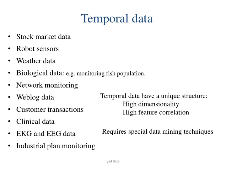
Temporal data • Stock market data • Robot sensors • Weather data • Biological data: e.g. monitoring fish population. • Network monitoring • Weblog data Temporal data have a unique structure: High dimensionality • Customer transactions High feature correlation • Clinical data Requires special data mining techniques • EKG and EEG data • Industrial plan monitoring Iyad Batal
Temporal data • Sequential data (no explicit time) vs. time series data – Sequential data e.g. : Gene sequences (we care about the order, but there is no explicit time!). • Real valued series vs. symbolic series – Symbolic series e.g.: customer transaction logs. • Regularly sampled vs irregularly sampled time series – Regularly sampled time series e.g.: stock data. – Irregularly sampled time series e.g.: weblog data, disc accesses. • Univariate vs multivariate – Mulitvarite time series e.g.: EEG data Example: clinical datasets are usually multivariate, real valued and irregularly sampled time series. Iyad Batal
Temporal Data Mining Tasks Classification Clustering Motif Discovery Rule Discovery Query by Content 10 A B C 0 50 0 1000 150 0 2000 2500 sup = 0.5 conf = 0.6 A B C 0 20 40 60 80 100 120 140 0 20 40 60 80 100 120 140 0 20 40 60 80 100 120 140 Anomaly Detection Visualization Iyad Batal
Temporal Data Mining • Hidden Markov Model (HMM) • Spectral time series representation – Discrete Fourier Transform (DFT) – Discrete Wavelet Transform (DWT) • Pattern mining – Sequential pattern mining – Temporal abstraction pattern mining Iyad Batal
Markov Models Rain Dry Dry Rain Dry { , , , } s s s • Set of states: 1 2 N • Process moves from one state to another generating a , , , , s s s sequence of states: 1 2 i i ik • Markov chain property: probability of each subsequent state depends only on what was the previous state: ( | , , , ) ( | ) P s s s s P s s 1 2 1 1 ik i i ik ik ik • Markov model parameter a o transition probabilities: ( | ) P s s ij i j o initial probabilities: ( ) P s i i Iyad Batal
Markov Model 0.3 0.7 Rain Dry 0.2 0.8 Two states : Rain and Dry. • • Transition probabilities: P(Rain|Rain)=0.3 , P(Dry|Rain)=0.7 , P(Rain|Dry)=0.2, P(Dry|Dry)=0.8 • Initial probabilities: say P(Rain)=0.4 , P(Dry)=0.6. • P({Dry, Dry, Rain, Rain} ) = P(Dry) P(Dry|Dry) P(Rain|Dry) P(Rain|Rain) = 0.6 * 0.8 * 0.2 * 0.3 Iyad Batal
Hidden Markov Model (HMM) Low High High Low Low Rain Dry Dry Rain Dry • States are not visible, but each state randomly generates one of M observations (or visible states) • Markov model parameter: M=(A, B, ) a o Transition probabilities: ( | ) P s s ij i j o Initial probabilities: ( ) P s i i o Emission probabilities: ( ) ( | ) b v P v s i m m i Iyad Batal
Hidden Markov Model (HMM) Initial probabilities: P(Low)=0.4 , P(High)=0.6 . 0.3 0.7 Low High 0.2 0.8 N T possible paths: 0.6 0.6 0.4 0.4 Exponential complexity! Rain Dry P({Dry,Rain} ) = P({Dry,Rain} , {Low,Low}) + P({Dry,Rain} , {Low,High}) + P({Dry,Rain} , {High,Low}) + P({Dry,Rain} , {High,High}) where first term is : P({Dry,Rain} , {Low,Low})= P(Low)*P(Dry|Low)* P(Low|Low)*P(Rain|Low) = 0.4*0.4*0.3*0.6 Iyad Batal
Hidden Markov Model (HMM) The Three Basic HMM Problems • Problem 1 (Evaluation): Given the HMM: M=(A, B, ) and the observation sequence O=o 1 o 2 ... o K , calculate the probability that model M has generated sequence O. Forward algorithm • Problem 2 (Decoding): Given the HMM: M=(A, B, ) and the observation sequence O=o 1 o 2 ... o K , calculate the most likely sequence of hidden states q 1 … q K that produced O. Viterbi algorithm Iyad Batal
Hidden Markov Model (HMM) The Three Basic HMM Problems • Problem 3 (Learning): Given some training observation sequences O and general structure of HMM (numbers of hidden and visible states), determine HMM parameters M=(A, B, ) that best fit the training data, that is maximizes P(O|M). Baum-Welch algorithm (EM) Iyad Batal
Hidden Markov Model (HMM) Forward algorithm Use Dynamic programming: Define the forward variable k (i) as the joint probability of the partial observation sequence o 1 o 2 ... o k and that the hidden state at time k is s i : k (i)= P(o 1 o 2 ... o k , q k = s i ) • Initialization: 1 (i)= P(o 1 , q 1 = s i ) = i b i (o 1 ) , 1<=i<=N. Complexity : N 2 T operations. • Forward recursion: k+1 (i)= P(o 1 o 2 ... o k+1 , q k+1 = s j ) = i P(o 1 o 2 ... o k+1 , q k = s i , q k+1 = s j ) = i P(o 1 o 2 ... o k , q k = s i ) a ij b j (o k+1 ) = [ i k (i) a ij ] b j (o k+1 ) , 1<=j<=N, 1<=k<=K-1. • Termination: P(o 1 o 2 ... o T ) = i P(o 1 o 2 ... o T , q T = s i ) = i T (i) Iyad Batal
Hidden Markov Model (HMM) Baum-Welch algorithm If training data has information about sequence of hidden states, then use maximum likelihood estimation of parameters: Number of transitions from state s j to state s i a ij = P(s i | s j ) = Number of transitions out of state s j Number of times observation v m occurs in state s i b i (v m ) = P(v m | s i ) = Number of times in state s i i = P(s i ) = Number of times state S i occur at time k=1. Iyad Batal
Hidden Markov Model (HMM) Baum-Welch algorithm Using an initial parameter instantiation, the algorithm iteratively re- estimates the parameters to improve the probability of generating the observations Expected number of transitions from state s j to state s i a ij = P(s i | s j ) = Expected number of transitions out of state s j Expected number of times observation v m occurs in state s i b i (v m ) = P(v m | s i ) = Expected number of times in state s i i = P(s i ) = Expected Number of times state S i occur at time k=1. The algorithm uses iterative expectation-maximization algorithm to find local optimum solution Iyad Batal
Temporal Data Mining • Hidden Markov Model (HMM) • Spectral time series representation – Discrete Fourier Transform (DFT) – Discrete Wavelet Transform (DWT) • Pattern mining – Sequential pattern mining – Temporal abstraction pattern mining Iyad Batal
DFT • Discrete Fourier transform (DFT) transforms the series from the time domain to the frequency domain. • Given a sequence x of length n, DFT produces n complex numbers: Remember that exp(j ϕ )=cos( ϕ ) + j sin( ϕ ). • DFT coefficients (X f ) are complex numbers: Im(X f ) is sine at frequency f and Re(X f ) is cosine at frequency f, but X 0 is always a real number. • DFT decomposes the signal into sine and cosine functions of several frequencies. • The signal can be recovered exactly by the inverse DFT: Iyad Batal
DFT • DFT can be written as a matrix operation where A is a n x n matrix: A is column-orthonormal. Geometric view: view series x as a point in n-dimensional space. • A does a rotation (but no scaling) on the vector x in n-dimensional complex space: – Does not affect the length – Does not affect the Euclidean distance between any pair of points Iyad Batal
DFT • Symmetry property: X f =(X n-f )* where * is the complex conjugate, therefore, we keep only the first half of the spectrum. • Usually, we are interested in the amplitude spectrum (|X f |) of the signal: • The amplitude spectrum is insensitive to shifts in the time domain • Computation: – Naïve: O(n 2 ) – FFT: O(n log n) Iyad Batal
DFT Example1: We show only half the spectrum because of the symmetry Very good compression! Iyad Batal
DFT Example2: the Dirac delta function. Horrible! The frequency leak problem Iyad Batal
SWFT • DFT assumes the signal to be periodic and have no temporal locality: each coefficient provides information about all time points. • Partial remedy: the Short Window Fourier Transform (SWFT) divides the time sequence into non-overlapping windows of size w and perform DFT on each window. • The delta function have restricted ‘frequency leak’. • How to choose the width w? – Long w gives good frequency resolution and poor time resolution. – Short w gives good time resolution and poor frequency resolution. Solution: let w be variable → Discrete Wavelet Transform (DWT) • Iyad Batal
DWT • DWT maps the signal into a joint time-frequency domain. • DWT hierarchically decomposes the signal using windows of different sizes (multi resolution analysis): – Good time resolution and poor frequency resolution at high frequencies. – Good frequency resolution and poor time resolution at low frequencies. Iyad Batal
DWT: Haar wavelets Initial condition: Iyad Batal
DWT: Haar wavelets Length of the series should be a power of 2: zero pad the series! The Haar transform: all the difference values d l,i at every level l and offset i (n-1) difference, plus the smooth component s L,0 at the last level Computational complexity is O(n) Iyad Batal
Recommend
More recommend
Explore More Topics
Stay informed with curated content and fresh updates.
