Technical Challenges Nikolaus Grigorieff Brandeis University - PowerPoint PPT Presentation
Technical Challenges Nikolaus Grigorieff Brandeis University Larson, The Far Side What Technical Challenges? 3.6 resolution Wolf et al. 2010 An Old Prophecy How many images must be averaged to reach near-atomic resolution? Theoretical
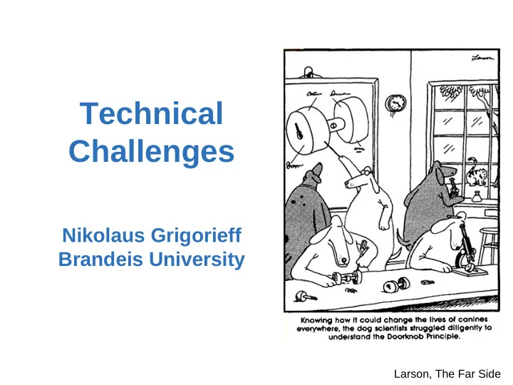
Technical Challenges Nikolaus Grigorieff Brandeis University Larson, The Far Side
What Technical Challenges? 3.6 Å resolution Wolf et al. 2010
An Old Prophecy How many images must be averaged to reach near-atomic resolution? Theoretical prediction (Henderson, Glaeser): a few thousand Papillomavirus L1 subunits averaged to reach 3.6 Å: 1.5 million!
Contrast and Noise 8.3 Å SNR 1/10 ≈ Bacteriorhodopsin
Aligning Small Particles 100 kDa Bacteriorhodopsin
B-Factor Analysis 0.5 native bR ln(image/diffraction amplitudes) native bR 0 (2.8 Å) DOC bR -0.5 B = 140 Å 2 -1 (200 kV, FEG, l. helium, -1.5 10 e - /Å 2 ) B = 180 Å 2 -2 (120 kV, tungsten -2.5 10 lipids filament, l. helium, -3 10 e - /Å 2 ) per bR -3.5 0 0.02 0.04 0.06 0.08 0.1 DOC bR Resolution [Å -2 ] 2.6 Å) B damage = 40 Å 2 (liquid helium) B detector = 70 Å 2 (film) → B total = 110 Å 2 6 lipids per bR Grigorieff et al. 1995
B-Factor Analysis 3.6 Å resolution 3,977 particles B damage = 60 Å 2 (liquid nitrogen) 60-fold icos. sym. 6-fold non-icos. sym. B detector = 70 Å 2 (film) B motion = 160 Å 2 (Campbell et al. 2012) Wolf et al. 2010 B alignment = 90 Å 2 (σ shift = 0.2 Å, σ rot = 0.2º, 12 σ defocus = 200 Å) Papillomavirus without 10 non-icosahedral averaging → B total = 380 Å 2 ln(amplitudes) (resolution = 4.4 Å) 8 B = 510 Å 2 6 B observed = 510 Å 2 B = 260 Å 2 4 → B unexplained = 130 Å 2 2 0 0.01 0.02 0.03 0.04 0.05 Resolution [Å -2 ]
B-Factor Analysis 3.6 Å resolution 3,977 particles 60-fold icos. sym. 6-fold non-icos. sym. → 24,000 “60-fold” particles Wolf et al. 2010 12 Papillomavirus without 10 non-icosahedral averaging ln(amplitudes) (resolution = 4.4 Å) 8 B = 510 Å 2 6 B = 260 Å 2 4 2 0 0.01 0.02 0.03 0.04 0.05 Resolution [Å -2 ] Rosenthal & Henderson 2003
The Challenges • Beam-induced motion & charging • Detector DQE • Beam damage • Alignment errors Larson, The Far Side
Better Sample Support Thin carbon support shows crinkling due to shrinking of the copper grid (0.3%) and paraffin crystals (1% – 2%) at liquid nitrogen temperature. Thick carbon (350 Å) reduces or eliminated movement. → Flatness and mechanical strength of the support film are important. Molybdenum grids may help. 60º tilt Glaeser et al. 2011
Movies Recorded with direct electron detector DE-12 (Direct Electron) Frame rate = 40 fps Dose/frame = 0.5 e - /Å 2 Duration = 1.5 s No. of frames = 60 Total dose = 30 e - /Å 2 1 movie = 720 MB (1 byte/pixel) → Data Tsunami! Brilot et al. 2012
Frame Alignment 60-frame average 60-frame average (no alignment) (translational alignment) Brilot et al. 2012
Paraxial Charge Compensation C2 Berriman & Rosenthal 2012
The Challenges • Beam-induced motion & charging Contrast • Detector DQE • Beam coherence • Alignment errors
Improving Contrast • Better detectors • Low voltage • Phase plate • Inelastic scattering • Astigmatism Larson, The Far Side
Direct Electron Detectors 300 kV Chris Booth (Gatan) Benjamin Bammes (Direct Electron) Panel discussion (David Agard) McMullan & Henderson, 2009
Perfect Detector Δ = 22% McMullan & Henderson, 2009 Gatan webpage, 2012
Low Voltage Trimers of HIV gp140 in ice M = 420 kDa 80 kV 20 e - /Å 2 DQE of film and scintillator-based cameras improved at lower voltage 500 Å Harris et al 2011
Phase Plate GroEL in ice 20 nm 20 nm Defocus contrast Zernike phase plate Wah Chiu, Bob Glaeser Danev & Nagayama 2008
Phase Plate with Lasers Elastic Compton scattering Spherical resonant cavity 40 W laser with λ = 2 μm Müller et al. 2010
Inelastic Scattering Unfiltered 0 eV 25 eV 300 kV, 6 μm underfocus, 15 eV energy window Assuming 700 Å sample thickness: Electrons scattered elastically: 9% scattered inelastically: 18% → C c correctors will increase image contrast. Chen Xu (unpublished)
Astigmatic CTF Hemocyanine 3.8 MDa D 2 symmetry Martin et al. 2007 DF 1 = 1000 Ǻ, DF 2 = 14000 Ǻ Grant & van Heel (unpublished)
Potential Improvements 1 1 1 B=520 Å 2 B=520 Å 2 B=520 Å 2 0.8 0.8 0.8 B=360 Å 2 B=360 Å 2 B damage = 60 Å 2 B=290 Å 2 Envelope Envelope Envelope 0.6 0.6 0.6 B detector = 70 Å 2 0.4 0.4 0.4 B motion = 160 Å 2 B alignment = 90 Å 2 0.2 0.2 0.2 0 0 0 0 0 0 0.05 0.05 0.05 0.1 0.1 0.1 0.15 0.15 0.15 0.2 0.2 0.2 0.25 0.25 0.25 0.3 0.3 0.3 Factor @ 3.5 Å: Resolution[Å -1 ] Resolution[Å -1 ] Resolution[Å -1 ] 110 12,000 x signal
The Challenges • Beam-induced motion & charging • Detector DQE • Beam damage • Alignment errors Larson, The Far Side
Optimal Dose 2.5 N e = 12 e - /Å 2 2 (50 Å resolution) SNR (arb. units) 1.5 N e = 6 e - /Å 2 (7 Å resolution) 1 19x 5x 0.5 B = 60 Å 2 N e = 1.2 e - /Å 2 B = 30 Å 2 (3 Å resolution) 0 0 5 10 15 20 25 30 Dose (electrons/Å 2 ) John Rubinstein Unwin & Henderson 1975; Hayward & Glaeser 1979; Stark et al. 1996, Baker et al. 2010
High-Dose Imaging 104 electrons/Å 2 24 electrons/Å 2 Voltage = 200 kV Defocus = 1.5 μm Flu hemagglutinin (2FK0, Stevens et al. 2006) Trimer = 180 kDa Melody Campbell Peter Lee (unpublished)
Thon Ring Patterns 6 Å No frame alignment With frame alignment Melody Campbell Peter Lee (unpublished)
Potential Improvements 1 1 1 1 B=520 Å 2 B=520 Å 2 B=520 Å 2 B=520 Å 2 0.8 0.8 0.8 0.8 B=360 Å 2 B=360 Å 2 B=360 Å 2 B damage = 30 Å 2 B=290 Å 2 B=290 Å 2 Envelope Envelope Envelope Envelope 0.6 0.6 0.6 0.6 B detector = 70 Å 2 B=260 Å 2 0.4 0.4 0.4 0.4 B motion = 160 Å 2 B alignment = 90 Å 2 0.2 0.2 0.2 0.2 0 0 0 0 0 0 0 0 0.05 0.05 0.05 0.05 0.1 0.1 0.1 0.1 0.15 0.15 0.15 0.15 0.2 0.2 0.2 0.2 0.25 0.25 0.25 0.25 0.3 0.3 0.3 0.3 Factor @ 3.5 Å: Resolution[Å -1 ] Resolution[Å -1 ] Resolution[Å -1 ] Resolution[Å -1 ] 200 40,000 x signal
The Challenges • Beam-induced motion & charging • Beam damage • Detector DQE • Alignment errors Larson, The Far Side
Dealing With Noise 100 kDa Bacteriorhodopsin
Maximum Likelihood Correlation alignment N = 4000 SNR = 1/200 ML estimation Sjors Scheres Sigworth 1998
ML Classification SNR = 1/50 Difference N = 2000 map Sjors Scheres Pawel Penczek Correlation alignment
All Things Considered • Accurate modeling of all parameters – CTF, envelope, variability … • Statistical models – noise models, parameter distributions, weighting … • Score dependent on all known facts/data – cross-linking, homology, total mass … • Reproducibility tests – multiple starts, consistency checks … • Large data sets – automation
Helical Processing with Frealix Emphasis on flexible filaments Rotational alignment of a single crossover (amyloid fibrils) Correlation in neighboring areas Full-filament processing helps find correct alignment (no segment boxing) Other filament types (TMV, microtubules) Constraints during image processing low score (persistence length...) high score Alexis Rohou, unpublished
Computer Games (Doom et al.) 10 6 7 10 5 10 6 10 10 4 Voxel MIPS 5 10 1000 4 10 100 10 1000 1990 1995 2000 2005 2010 Year
Sample Limitations • Sample heterogeneity/stability – biochemistry – new algorithms • Transient complexes – affinity grids, streptavidin crystals • Detergent and lipid – amphipol, GLC/GDN Larson, The Far Side – amphiphilic β-strand peptides • Low molecular weight Holger Stark Debbie Kelly
Scaffolds Yifan Cheng HA 6-helix bundle adapter VP7 Ni-NTA nanogold Rotavirus DLP His-tagged flu hemagglutinin Junhua Pan, Yuhang Liu, unpublished unpublished
Thank You!
Recommend
More recommend
Explore More Topics
Stay informed with curated content and fresh updates.

