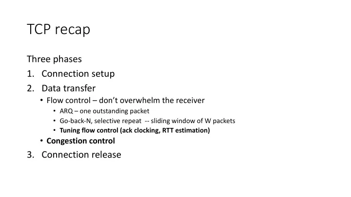
TCP recap Three phases 1. Connection setup 2. Data transfer Flow - PowerPoint PPT Presentation
TCP recap Three phases 1. Connection setup 2. Data transfer Flow control dont overwhelm the receiver ARQ one outstanding packet Go-back-N, selective repeat -- sliding window of W packets Tuning flow control (ack
TCP recap Three phases 1. Connection setup 2. Data transfer • Flow control – don’t overwhelm the receiver • ARQ – one outstanding packet • Go-back-N, selective repeat -- sliding window of W packets • Tuning flow control (ack clocking, RTT estimation) • Congestion control 3. Connection release
ACK Clocking
Sliding Window ACK Clock • Typically, the sender does not know B or D • Each new ACK advances the sliding window and lets a new segment enter the network • ACK s “clock” data segments 20 19 18 17 16 15 14 13 12 11 Data Ack 1 2 3 4 5 6 7 8 9 10 CSE 461 University of Washington 3
Benefit of ACK Clocking • Consider what happens when sender injects a burst of segments into the network Queue Slow (bottleneck) link Fast link Fast link CSE 461 University of Washington 4
Benefit of ACK Clocking (2) • Segments are buffered and spread out on slow link Segments “spread out” Fast link Slow (bottleneck) link Fast link CSE 461 University of Washington 5
Benefit of ACK Clocking (3) • ACK s maintain the spread back to the original sender Slow link Acks maintain spread CSE 461 University of Washington 6
Benefit of ACK Clocking (4) • Sender clocks new segments with the spread • Now sending at the bottleneck link without queuing! Segments spread Queue no longer builds Slow link CSE 461 University of Washington 7
Benefit of ACK Clocking (4) • Helps run with low levels of loss and delay! • The network smooths out the burst of data segments • ACK clock transfers this smooth timing back to sender • Subsequent data segments are not sent in bursts so do not queue up in the network CSE 461 University of Washington 8
TCP Uses ACK Clocking • TCP uses a sliding window because of the value of ACK clocking • Sliding window controls how many segments are inside the network • TCP only sends small bursts of segments to let the network keep the traffic smooth CSE 461 University of Washington 9
Problem • Sliding window has pipelining to keep network busy • What if the receiver is overloaded? Arg … Streaming video Big Iron Wee Mobile CSE 461 University of Washington 10
Receiver Sliding Window • Consider receiver with W buffers • LAS= LAST ACK SENT • app pulls in-order data from buffer with recv() call Sliding W=5 Window 5 6 7 5 5 5 5 5 2 3 .. 3 .. Finished Acceptable .. Too high LAS seq. number CSE 461 University of Washington 11
Receiver Sliding Window (2) • Suppose the next two segments arrive but app does not call recv() W=5 5 6 7 5 5 5 5 5 2 3 .. 3 .. Finished Acceptable .. Too high LAS seq. number CSE 461 University of Washington 12
Receiver Sliding Window (3) • Suppose the next two segments arrive but app does not call recv() • LAS rises, but we can’t slide window! W=5 5 6 7 5 5 5 5 5 2 3 .. 3 .. Finished Acked .. Too high LAS seq. number CSE 461 University of Washington 13
Receiver Sliding Window (4) • Further segments arrive (in order) we fill buffer • Must drop segments until app recvs! Nothing W=5 Acceptable! 5 6 7 5 5 5 5 5 2 3 .. 3 .. Finished Acked .. Too high LAS seq. number CSE 461 University of Washington 14
Receiver Sliding Window (5) • App recv() takes two segments • Window slides (phew) W=5 Acceptable 5 6 7 5 5 5 5 5 2 3 .. 3 Acked .. Finished .. LAS seq. number CSE 461 University of Washington 15
Flow Control • Avoid loss at receiver by telling sender the available buffer space • WIN =#Acceptable, not W (from LAS) W=5 Acceptable 5 6 7 5 5 5 5 5 2 3 .. 3 Acked .. Finished .. LAS seq. number CSE 461 University of Washington 16
Flow Control (2) • Sender uses lower of the sliding window and flow control window ( WIN ) as the effective window size W=3 Acceptable 5 6 7 5 5 5 5 5 2 3 .. 3 .. Finished Acked .. Too high LAS seq. number CSE 461 University of Washington 17
Flow Control (3) • TCP-style example • SEQ / ACK sliding window • Flow control with WIN • SEQ + length < ACK + WIN • 4KB buffer at receiver • Circular buffer of bytes CSE 461 University of Washington 18
Topic • How to set the timeout for sending a retransmission • Adapting to the network path Lost? Network CSE 461 University of Washington 19
Retransmissions • With sliding window, detecting loss with timeout • Set timer when a segment is sent • Cancel timer when ack is received • If timer fires, retransmit data as lost Retransmit! CSE 461 University of Washington 20
Timeout Problem • Timeout should be “just right” • Too long à inefficient network capacity use • Too short à spurious resends waste network capacity • But what is “just right”? • Easy to set on a LAN (Link) • Short, fixed, predictable RTT • Hard on the Internet (Transport) • Wide range, variable RTT CSE 461 University of Washington 21
Example of RTTs BCN à SEA à BCN 1000 900 Round Trip Time (ms) 800 700 600 500 400 300 200 100 0 0 20 40 60 80 100 120 140 160 180 200 Seconds CSE 461 University of Washington 22
Example of RTTs (2) BCN à SEA à BCN 1000 900 Variation due to queuing at routers, Round Trip Time (ms) changes in network paths, etc. 800 700 600 500 400 300 200 Propagation (+transmission) delay ≈ 2D 100 0 0 20 40 60 80 100 120 140 160 180 200 Seconds CSE 461 University of Washington 23
Example of RTTs (3) 1000 Timer too high! 900 Round Trip Time (ms) 800 Need to adapt to the 700 network conditions 600 500 Timer too low! 400 300 200 100 0 0 20 40 60 80 100 120 140 160 180 200 Seconds CSE 461 University of Washington 24
Adaptive Timeout • Smoothed estimates of the RTT (1) and variance in RTT (2) • Update estimates with a moving average 1. SRTT N+1 = 0.9*SRTT N + 0.1*RTT N+1 2. Svar N+1 = 0.9*Svar N + 0.1*|RTT N+1 – SRTT N+1 | • Set timeout to a multiple of estimates • To estimate the upper RTT in practice • TCP Timeout N = SRTT N + 4*Svar N CSE 461 University of Washington 25
Example of Adaptive Timeout 1000 900 800 700 RTT (ms) 600 SRTT 500 400 300 200 Svar 100 0 0 20 40 60 80 100 120 140 160 180 200 Seconds CSE 461 University of Washington 26
Example of Adaptive Timeout (2) 1000 Early 900 timeout Timeout (SRTT + 4*Svar) 800 700 RTT (ms) 600 500 400 300 200 100 0 0 20 40 60 80 100 120 140 160 180 200 Seconds CSE 461 University of Washington 27
Adaptive Timeout (2) • Simple to compute, does a good job of tracking actual RTT • Little “headroom” to lower • Yet very few early timeouts • Turns out to be important for good performance and robustness CSE 461 University of Washington 28
Congestion
TCP to date: • We can set up and tear connections • Connection establishment and release handshakes • Keep the sending and receiving buffers from overflowing (flow control) What’s missing?
Network Congestion • A “traffic jam” in the network • Later we will learn how to control it What’s the hold up? Network CSE 461 University of Washington 31
Congestion Collapse in the 1980s • Early TCP used fixed size window (e.g., 8 packets) • Initially fine for reliability • But something happened as the network grew • Links stayed busy but transfer rates fell by orders of magnitude! CSE 461 University of Washington 32
Nature of Congestion • Routers/switches have internal buffering Input . . . Output . . . . . . . . . Fabric Output Buffer Input Buffer CSE 461 University of Washington 33
Nature of Congestion (2) • Simplified view of per port output queues • Typically FIFO (First In First Out), discard when full Router Router = Queued (FIFO) Queue Packets CSE 461 University of Washington 34
Nature of Congestion (3) • Queues help by absorbing bursts when input > output rate • But if input > output rate persistently, queue will overflow • This is congestion • Congestion is a function of the traffic patterns – can occur even if every link has the same capacity CSE 461 University of Washington 35
Effects of Congestion • What happens to performance as we increase load?
Effects of Congestion (2) • What happens to performance as we increase load?
Effects of Congestion (3) • As offered load rises, congestion occurs as queues begin to fill: • Delay and loss rise sharply with load • Throughput < load (due to loss) • Goodput << throughput (due to spurious retransmissions) • None of the above is good! • Want network performance just before congestion CSE 461 University of Washington 38
TCP Tahoe/Reno • TCP extensions and features we will study: • AIMD • Fair Queuing • Slow-start • Fast Retransmission • Fast Recovery CSE 461 University of Washington 40
TCP Timeline TCP Reno (Jacobson, ‘90) TCP/IP “flag day” 3-way handshake (BSD Unix 4.2, ‘83) (Tomlinson, ‘75) TCP Tahoe TCP and IP (Jacobson, ’88) (RFC 791/793, ‘81) Origins of “TCP” (Cerf & Kahn, ’74) Congestion collapse 1988 Observed, ‘86 1970 1975 1980 1985 1990 . . . Congestion control Pre-history CSE 461 University of Washington 41
Recommend
More recommend
Explore More Topics
Stay informed with curated content and fresh updates.
