Taylor Models and Their Applications Martin Berz and Kyoko Makino - PowerPoint PPT Presentation
Taylor Models and Their Applications Martin Berz and Kyoko Makino Department of Physics and Astronomy Michigan State University Contributions: Alex Wittig (MSU) R. Armellin, P. Di Lizia (Politecnico di Milano) Outline Motivation
Taylor Models and Their Applications Martin Berz and Kyoko Makino Department of Physics and Astronomy Michigan State University Contributions: Alex Wittig (MSU) R. Armellin, P. Di Lizia (Politecnico di Milano)
Outline • Motivation • Introduction to Taylor models Basics. Arithmetic. Comparisons with interval computations. • Applications – Demonstrate with examples — Range bounding Moore’s simple 1D function — Global optimizations Moore’s simple 1D function. Normal form defect functions. — ODE integrations The Volterra equations. Near earth asteroid Apophis. The Lorenz equations.[Long time integrations, Poincare pro- jections, covering huge size initial conditions, manifolds] • Work in progress
Introduction Taylor model (TM) methods were originally developed for a practical problem from nonlinear dynamics, range bounding of normal form defect functions. • Functions consist of code lists of 10 4 to 10 5 terms • Have about the worst imaginable cancellation problem • Are obtained via validated integration of large initial condition boxes. Originally nearly universally considered intractable by the community. But ... a small challenge goes a long way towards generating new ideas! Idea: represent all functional dependencies as a pair of a polynomial P and a remainder bound I introduce arithmetic, and a new ODE solver. Obtain the following properties: • The ability to provide enclosures of any function given by a fi nite com- puter code list by a Taylor polynomial and a remainder bound with a sharpness that scales with order ( n + 1) of the width of the domain. • The ability to alleviate the dependency problem in the calculation. • The ability to scale favorable to higher dimensional problems.
Find guaranteed bound of such functions ===> The original motivation of Taylor models
Motion in the Tevatron Speed of Light: 3x10 8 m/sec • Circumference: 6.28x10 3 m • 4x10 4 revs/sec. Need to store about 10 hours, or 4x10 5 sec • 2x10 10 revolutions total. • 10,000 magnets in ring 2x10 14 contacts with fields! • Extremely challenging computationally •Need for several State-Of-The-Art Methods: •Phase Space Maps •Perturbation Theory •Lyapunov- and other Stability Theories •High-Performance Verified Methods
Bounds Estimates RDA Interval Method Taylor Model Method f U f R I f �� �� �� �� P f f L a a b b R Bounds: [f ] ,f Bounds: P +I L U f f : Polynomial P f R : Remainder Bounds I f
Interval Arithmetic A method to perform guaranteed calculations on computer by pre- senting all numbers by intervals. [ a ] + [ ] = [ a + + ] [ a ] − [ ] = [ a − − ] [ a ] · [ ] = [min( a a ) max( a a )] [ a ] / [ ] = [min( a/ a/ / / ) max( a/ a/ / / )] Not a group because [ a ] − [ ] 6 = [0 0] unless a = = . In particular, [ a ] − [ a ] = [ a − − a ] [ a ] / [ a ] = [min(1 a/ /a ) max(1 a/ /a )] Thus, operations lead to over estimation, which can become large with time to blow up.
Moore’s Simple 1D Function f ( x ) = 1 + x 5 − x 4 . Study on [0 , 1] . Trivial-looking, but dependency and high order. Assumes shallow min at 0 . 8 . y y 1 0.98 0.96 0.94 0.92 0 0.25 0.5 0.75 1 x x
Moore 1D function f(x)=x^5-x^4+1 in [0,1] 1.02 1 0.98 0.96 0.94 0.92 0.9 0 0.2 0.4 0.6 0.8 1
Moore 1D function f(x)=x^5-x^4+1 in [0,1]. Bounding by 16 intervals 1.3 1.2 1.1 1 0.9 0.8 0.7 0 0.2 0.4 0.6 0.8 1
Moore 1D function f(x)=x^5-x^4+1 in [0,1]. Bounding by 128 intervals 1.3 1.2 1.1 1 0.9 0.8 0.7 0 0.2 0.4 0.6 0.8 1
Moore 1D function f(x)=x^5-x^4+1 in [0,1]. Bounding by 128 intervals 1.02 1 0.98 0.96 0.94 0.92 0.9 0 0.2 0.4 0.6 0.8 1
Moore 1D function f(x)=x^5-x^4+1 in [0,1]. Bounding by 256 intervals 1.02 1 0.98 0.96 0.94 0.92 0.9 0 0.2 0.4 0.6 0.8 1
Moore 1D function f(x)=x^5-x^4+1 in [0,1]. Bounding by 512 intervals 1.02 1 0.98 0.96 0.94 0.92 0.9 0 0.2 0.4 0.6 0.8 1
Moore 1D function f(x)=x^5-x^4+1 in [0,1]. Bounding by 1024 intervals 1.02 1 0.98 0.96 0.94 0.92 0.9 0 0.2 0.4 0.6 0.8 1
De fi nitions - Taylor Models and Operations We begin with a review of the de fi nitions of the basic operations. De fi nition (Taylor Model) Let f : D ⊂ R v → R be a function that is ( n +1) times continuously partially di ff erentiable on an open set containing the domain v -dimensional domain D. Let x 0 be a point in D and P the n -th order Taylor polynomial of f around x 0 . Let I be an interval such that f ( x ) ∈ P ( x − x 0 ) + I for all x ∈ D. Then we call the pair ( P, I ) an n -th order Taylor model of f around x 0 on D. De fi nition (Addition and Multiplication) Let T 1 , 2 = ( P 1 , 2 , I 1 , 2 ) be n -th order Taylor models around x 0 over the domain D . We de fi ne T 1 + T 2 = ( P 1 + P 2 , I 1 + I 2 ) T 1 · T 2 = ( P 1 · 2 , I 1 · 2 ) where P 1 · 2 is the part of the polynomial P 1 · P 2 up to order n and I 1 · 2 = B ( P e ) + B ( P 1 ) · I 2 + B ( P 2 ) · I 1 + I 1 · I 2 where P e is the part of the polynomial P 1 · P 2 of orders ( n + 1) to 2 n , and B ( P ) denotes a bound of P on the domain D. We demand that B ( P ) is at least as sharp as direct interval evaluation of P ( x − x 0 ) on D.
De fi nitions - Taylor Model Intrinsics De fi nition (Intrinsic Functions of Taylor Models) Let T = ( P, I ) be a Taylor model of order n over the v -dimensional domain D = [ a, b ] around the point x 0 . We de fi ne intrinsic functions for the Taylor models by performing various manipulations that will allow the computation of Taylor models for the intrinsics from those of the arguments. In the following, let f ( x ) ∈ P ( x − x 0 ) + I be any function in the Taylor model, and let c f = f ( x 0 ) , and ¯ f be de fi ned by ¯ f ( x ) = f ( x ) − c f . Likewise we de fi ne ¯ P by P ( x − x 0 ) = P ( x − x 0 ) − c f , so that ( ¯ ¯ P, I ) is a Taylor model for ¯ f. For the various intrinsics, we proceed as follows. Exponential. We fi rst write ¡ ¢ ¡ ¯ ¢ c f + ¯ exp( f ( x )) = exp f ( x ) = exp( c f ) · exp f ( x ) ½ f ( x ) + 1 f ( x )) 2 + · · · + 1 1 + ¯ 2!( ¯ k !( ¯ f ( x )) k = exp( c f ) · ¢¾ ¡ 1 f ( x )) k +1 exp ( k + 1)!( ¯ θ · ¯ + f ( x ) , where 0 < θ < 1 .
De fi nitions - Taylor Model Exponential, cont. Taking k ≥ n , the part ½ ¾ f ( x ) + 1 f ( x )) 2 + · · · + 1 1 + ¯ 2!( ¯ n !( ¯ f ( x )) n exp( c f ) · is merely a polynomial of ¯ f , of which we can obtain the Taylor model via Taylor model addition and multiplication. The remainder part of exp( f ( x )) , the expression ½ 1 ( n + 1)!( ¯ f ( x )) n +1 exp( c f ) · ¢¾ ¡ 1 f ( x )) k +1 exp ( k + 1)!( ¯ θ · ¯ + · · · + f ( x ) , will be bounded by an interval. First observe that since the Taylor polyno- mial of ¯ f does not have a constant part, the ( n + 1) -st through ( k + 1) -st P, I ) of ¯ powers of the Taylor model ( ¯ f will have vanishing polynomial part, and thus so does the entire remainder part. The remainder bound interval for the Lagrange remainder term
De fi nitions - Taylor Model Exponential, cont. ¡ ¢ 1 f ( x )) k +1 exp ( k + 1)!( ¯ θ · ¯ exp( c f ) f ( x ) can be estimated because, for any x ∈ D , ¯ P ( x − x 0 ) ∈ B ( ¯ P ) , and 0 < θ < 1 , and so ¡ ¢ ¡ ¢ k +1 f ( x )) k +1 exp ( ¯ θ · ¯ B ( ¯ f ( x ) ∈ P ) + I ¡ ¢ [0 , 1] · ( B ( ¯ × exp P ) + I ) . The evaluation of the “ exp ” term is mere standard interval arithmetic. In the actual implementation, one may choose k = n for simplicity, but it is not a priori clear which value of k would yield the sharpest enclosures.
De fi nitions - Taylor Model Arc Sine Arcsine. Under the condition ∀ x ∈ D, B ( P ( x − x 0 ) + I ) ⊂ ( − 1 , 1) , using an addition formula for the arcsine, we re-write q ³ ´ p 1 − c 2 1 − ( f ( x )) 2 arcsin( f ( x )) = arcsin( c f ) + arcsin f ( x ) · f − c f · . Utilizing that q p 1 − c 2 1 − ( f ( x )) 2 g ( x ) ≡ f ( x ) · f − c f · does not have a constant part, we have 5!( g ( x )) 5 + 3 2 · 5 2 3!( g ( x )) 3 + 3 2 arcsin( g ( x )) = g ( x ) + 1 ( g ( x )) 7 7! 1 ( k + 1)!( g ( x )) k +1 · arcsin ( k +1) ( θ · g ( x )) , + · · · + where p arcsin 0 ( a ) = 1 / arcsin 00 ( a ) = a/ (1 − a 2 ) 3 / 2 , 1 − a 2 , arcsin (3) ( a ) = (1 + 2 a 2 ) / (1 − a 2 ) 5 / 2 , ...
Recommend
More recommend
Explore More Topics
Stay informed with curated content and fresh updates.
