TagProp: Discriminative Metric Learning in Nearest Neighbour Models - PowerPoint PPT Presentation
Introduction Metric Learning Data Sets and Evaluation Results Conclusion TagProp: Discriminative Metric Learning in Nearest Neighbour Models for Image Auto-Annotation Guillaumin, Mensink, Verbeek, Schmid Daniel Rios-Pavia, Thomas
Introduction Metric Learning Data Sets and Evaluation Results Conclusion TagProp: Discriminative Metric Learning in Nearest Neighbour Models for Image Auto-Annotation Guillaumin, Mensink, Verbeek, Schmid Daniel Rios-Pavia, Thomas Vincent-Sweet UJF, Ensimag January 14, 2011
Introduction Metric Learning Data Sets and Evaluation Results Conclusion Layout Introduction 1 Metric Learning 2 Tag prediction Rank-based Distance-based Sigmoidal modulation Data Sets and Evaluation 3 Feature Extraction Data Sets Evaluation Results 4 Conclusion 5
Introduction Metric Learning Data Sets and Evaluation Results Conclusion Layout Introduction 1 Metric Learning 2 Tag prediction Rank-based Distance-based Sigmoidal modulation Data Sets and Evaluation 3 Feature Extraction Data Sets Evaluation Results 4 Conclusion 5
Introduction Metric Learning Data Sets and Evaluation Results Conclusion TagProp: Tag Propagation Aim: Tag images automatically through keyword relevance prediction Applications: Image annotation Image search
Introduction Metric Learning Data Sets and Evaluation Results Conclusion Auto-Annotation Example
Introduction Metric Learning Data Sets and Evaluation Results Conclusion Layout Introduction 1 Metric Learning 2 Tag prediction Rank-based Distance-based Sigmoidal modulation Data Sets and Evaluation 3 Feature Extraction Data Sets Evaluation Results 4 Conclusion 5
Introduction Metric Learning Data Sets and Evaluation Results Conclusion Predicting Tag Relevance Propagate annotations from training images to new images Use metric learning instead of fixed metric or ad-hoc combinations of metrics
Introduction Metric Learning Data Sets and Evaluation Results Conclusion Weighted Nearest Neighbour Tag Prediction Tags are either absent or present ( i : image w : word) y iw ∈ {− 1 , +1 }
Introduction Metric Learning Data Sets and Evaluation Results Conclusion Weighted Nearest Neighbour Tag Prediction Tags are either absent or present ( i : image w : word) y iw ∈ {− 1 , +1 } Tag presence prediction p ( y iw = +1): � p ( y iw = +1) = π ij p ( y iw = +1 | j ) j � 1 − ǫ for y jw = +1 p ( y iw = +1 | j ) = otherwise ǫ with π ij the weight of training image j for predictions for image i .
Introduction Metric Learning Data Sets and Evaluation Results Conclusion Weighted Nearest Neighbour Tag Prediction Tags are either absent or present ( i : image w : word) y iw ∈ {− 1 , +1 } Tag presence prediction p ( y iw = +1): � p ( y iw = +1) = π ij p ( y iw = +1 | j ) j � 1 − ǫ for y jw = +1 p ( y iw = +1 | j ) = otherwise ǫ with π ij the weight of training image j for predictions for image i . � π ij ≥ 0 and π ij = 1 j
Introduction Metric Learning Data Sets and Evaluation Results Conclusion Weighted Nearest Neighbour Tag Prediction Estimation of parameters that control weights π iw Maximize the log-likelihood of predictions: � L = c iw log p ( y iw ) i , w where c iw is the cost taking into account presence/absence imbalance: c iw = 1 n + if y iw = +1 n + being the total number of positive labels. (same for n − )
Introduction Metric Learning Data Sets and Evaluation Results Conclusion Example
Introduction Metric Learning Data Sets and Evaluation Results Conclusion Example � 1 − ǫ for y jw = +1 p ( y iw = +1 | j ) = otherwise ǫ
Introduction Metric Learning Data Sets and Evaluation Results Conclusion Rank-based Weighting Fixed weight for the k-th neighbor: π iw = γ k K neighbors → K parameters L is concave with respect to { γ k } EM-algorithm Projected gradient descent Effective neighborhood size is set automatically 0.25 0.2 Weight 0.15 0.1 0.05 0 0 5 10 15 20 Neighbor Rank
Introduction Metric Learning Data Sets and Evaluation Results Conclusion Distance-based Weighting Weights given by visual distance d θ exp( − d θ ( i , j )) π ij = � k exp( − d θ ( i , k )) where θ are the parameters we want to optimize. Weights depend smoothly on distance important if distance adjustment is needed during training. Only one parameter per base distance
Introduction Metric Learning Data Sets and Evaluation Results Conclusion Distance-based Weighting Choices for d θ include (not exhaustive): A fixed distance d with a positive scale factor d w ( i , j ) = w T d ij with d ij a vector of base distances w contains the positive coefficients of the distance combination Mahalanobis distance As before, projected gradient algorithm to maximize log-likelihood and learn the distance combination.
Introduction Metric Learning Data Sets and Evaluation Results Conclusion Boosting the Recall of Rare Words Keywords with low frequency in database have low recall Mass of neighbors too small Systematic low relevance of keyword Boosting needed.
Introduction Metric Learning Data Sets and Evaluation Results Conclusion Sigmoidal modulation Word-specific logistic discriminant model ’dynamic range’ adjusted per word p ( y iw = +1) = σ ( α w x iw + β w )
Introduction Metric Learning Data Sets and Evaluation Results Conclusion Sigmoidal modulation Word-specific logistic discriminant model ’dynamic range’ adjusted per word p ( y iw = +1) = σ ( α w x iw + β w ) 1 with σ ( z ) = � � 1 + exp( − z ) and x iw = � j π ij y iw
Introduction Metric Learning Data Sets and Evaluation Results Conclusion Sigmoidal modulation Word-specific logistic discriminant model ’dynamic range’ adjusted per word p ( y iw = +1) = σ ( α w x iw + β w ) 1 with σ ( z ) = � � 1 + exp( − z ) and x iw = � j π ij y iw Adds 2 parameters for each word { α w , β w } Optimize through training (alternating maximization) { α w , β w } neighbour weights π ij
Introduction Metric Learning Data Sets and Evaluation Results Conclusion Sigmoid function
Introduction Metric Learning Data Sets and Evaluation Results Conclusion Layout Introduction 1 Metric Learning 2 Tag prediction Rank-based Distance-based Sigmoidal modulation Data Sets and Evaluation 3 Feature Extraction Data Sets Evaluation Results 4 Conclusion 5
Introduction Metric Learning Data Sets and Evaluation Results Conclusion Feature Extraction 15 image representations:
Introduction Metric Learning Data Sets and Evaluation Results Conclusion Feature Extraction 15 image representations: Global GIST descriptor Global colour histograms RGB, HSV, LAB 16 bin quantization Bag-of-Words histograms SIFT and Hue descriptors Dense grid and Harris-Laplacian interest points K-means quantization
Introduction Metric Learning Data Sets and Evaluation Results Conclusion Feature Extraction 15 image representations: Global GIST descriptor Global colour histograms RGB, HSV, LAB 16 bin quantization Bag-of-Words histograms SIFT and Hue descriptors Dense grid and Harris-Laplacian interest points K-means quantization 3x1 spatial partitioning for BoW and colour histograms
Introduction Metric Learning Data Sets and Evaluation Results Conclusion Corel 5k 5000 images (landscape, animals...) max 5 tags per image (avg=3) Vocabulary size = 260
Introduction Metric Learning Data Sets and Evaluation Results Conclusion ESP Game 20’000 images subset - 60k total (drawings, photos...) max 15 tags per image (avg=5) Vocabulary size = 268 Players annotate images in pairs
Introduction Metric Learning Data Sets and Evaluation Results Conclusion IAPR TC12 20’000 images (tourist photos, sports...) max 23 tags per image (avg=6) Vocabulary size = 291 Natural language processing from descriptive text
Introduction Metric Learning Data Sets and Evaluation Results Conclusion Evaluation Method Compute measures per keyword, then average Annotate images with top 5 keywords Recall (nr. annotated/nr. in DB) Precision (nr. correctly annotated/nr.annotated) N+ (nr. words with recall > 0) Retrieval (search) Rank results according to query keyword presence probability Precision for n w images (nr. ground truth images with w ) Mean Average Precision ( mAP ) and Break-Even Point ( BEP )
Introduction Metric Learning Data Sets and Evaluation Results Conclusion Layout Introduction 1 Metric Learning 2 Tag prediction Rank-based Distance-based Sigmoidal modulation Data Sets and Evaluation 3 Feature Extraction Data Sets Evaluation Results 4 Conclusion 5
Introduction Metric Learning Data Sets and Evaluation Results Conclusion Results: Annotation Distance > Rank
Introduction Metric Learning Data Sets and Evaluation Results Conclusion Results: Annotation Distance > Rank Sigmoid improves recall, loses precision
Introduction Metric Learning Data Sets and Evaluation Results Conclusion Results: Annotation Distance > Rank Sigmoid improves recall, loses precision Metric Learning gives significantly better results!
Introduction Metric Learning Data Sets and Evaluation Results Conclusion Results Improvement
Introduction Metric Learning Data Sets and Evaluation Results Conclusion Results: Recall All- BEP Difficult Single Multi Easy All PAMIR [7] 26 34 26 43 22 17 WN 32 40 31 49 28 24 σ WN 31 41 30 49 27 23 WN-ML 36 43 35 53 32 27 σ WN-ML 36 46 35 55 32 27 4. Comparison of WN-ML and PAMIR in terms of
Recommend
More recommend
Explore More Topics
Stay informed with curated content and fresh updates.
