Table of Contents 1. Motivation and Aims 2. Classification and - PDF document
27-10-17 Experiments in Fluid Mechanics ExFM 2017 Multiscale Modal Analysis of Experimental and Numerical Data Miguel. A. Mendez 1* , Mikhael Balabane 2 , Jean-Marie Buchlin 1 1 von Karman Institute for Fluid Dynamics, Rhode-St-Gense, Belgium 2
27-10-17 Experiments in Fluid Mechanics ExFM 2017 Multiscale Modal Analysis of Experimental and Numerical Data Miguel. A. Mendez 1* , Mikhael Balabane 2 , Jean-Marie Buchlin 1 1 von Karman Institute for Fluid Dynamics, Rhode-St-Genèse, Belgium 2 Laboratoire Analyse Geometrie et Applications, Paris 13, France Warsaw, Poland, 23-24 October, 2017 Table of Contents 1. Motivation and Aims 2. Classification and Algebra of Decompositions 3. Synthetic Test Cases 4. The Multiscale Proper Orthogonal Decomposition 4.1 Fourier Spectra and Eigenvalue Spectra 4.2 Multiresolution via Discrete Wavelets 4.3 The Gram-Schmidt Re-Assembly 5. Numerical and Experimental Test Cases 6. Conclusions 1
27-10-17 Motivation and Aims 1/51 Given a dataset D, we are interested only in a portion of the information it contains: Something Else Dataset Information Where and are the spatial and the temporal resolutions Example 1: Numerical Simulation of the 2D vorticity-streamline equation Where are the dominant sources of vorticity? How do they evolve in time and how do they interact? Mendez et al, ICNAAM 2017 Motivation and Aims 2/51 Given a dataset D, we are interested only in a portion of the information it contains: Dataset Information Something Else Where and are the spatial and the temporal resolutions Example 2: TR-PIV of an Oscillating Gas Jet Impinging on a Pulsing Interface What are the flow structures associated with the pulsation of the interface? What are those linked to the jet oscillation? Mendez et al, Exp Therm Fluid Sci 2017 2
27-10-17 What is a Decomposition ? 3/51 Decomposing means ‘to break down’ into constituent simpler parts, e.g.: Dataset Information Something Else Each of part has its own spatial and temporal evolution, and it is referred to as mode. We search for modes that can be written in a variable separated and normalized form: Spatial structure Energy Contribution Temporal Evolution Unitary energy structures/evolutions The most common decomposition is the Time-Discrete Fourier Transform (TDFT) where the temporal evolution of each mode is assumed to be harmonic: with and In order to have a frequency span Table of Contents 1. Motivation and Aims 2. Classification and Algebra of Decompositions 3. Synthetic Test Cases 4. The Multiscale Proper Orthogonal Decomposition 4.1 Fourier Spectra and Eigenvalue Spectra 4.2 Multiresolution via Discrete Wavelets 4.3 The Gram-Schmidt Re-Assembly 5. Numerical and Experimental Test Cases 6. Conclusions 3
27-10-17 The Algebra of any Decomposition 4/51 It is now useful to see a discrete decomposition from an algebraic point of view. At the scope assume we organize each snapshot into a column vector and we do the same for the spatial and the temporal structure of each mode: Data Matrix Spatial Structures Energy Contribution Temporal Evolutions The Algebra of any Decomposition 5/51 All the decomposition will therefore be written via matrix multiplication: Eq 1 To close the problem, one must set constraints in the spatial or in the temporal bases. Inferred (Unsupervised) Pre-Defined (Supervised) Proper Orthogonal Analytical Decomposition (POD) (Eigen-Functions) ‘ad hoc’ Fourier exponentials Dynamic Mode Fourier exponentials Legendre Polynomials Decomposition (DMD) Wavelets Chebyshev Polynomials Spectral Proper Bessel Functions Orthogonal Decomposition (SPOD) 4
27-10-17 The fundamental Classes 6/51 Eq 1 Energy Based: POD Mixed: SPOD Frequency Based: DMD ( M Sieber , 2015) (Schmidt, Rowley, 2009) (Lumley,1967) Goal: Goal: Goal: Minimize the number of Mixing 1 and 2 Harmonic Modes mode required Advantage: Advantage: Advantage: Good blending Spectral separation between POD/DFT Energy Optimality Pitfalls: Pitfalls: Pitfalls: Possible Spectral Mixing Possible poor Poor convergence, convergence and possible finite blow-ups lost of data inference The fundamental Classes: POD 7/51 Eq 1 Energy Based: POD We assume that both spatial and temporal dependencies form an orthonormal set. For a real dataset, orthonormality reads Therefore these bases are the set of eigenvectors of the covariance matrices, and the associated energies are the square roots of the corresponding eigenvectors The POD decomposition in Eq 1 becomes simply the Singular Value Decomposition (SVD) of the dataset D. The energy optimality is guaranteed by the Eckart-Young theorem. PROBLEM : Eigenvectors are unique up to repeated singular values 5
27-10-17 The fundamental Classes: DFT/DMD 8/51 Eq 1 Frequency Based: DMD As for the DFT, the DMD the temporal basis has a Vandermonde form: DFT: DMD: powers of a real, fundamental frequency Complex frequencies of the system with The fundamental Classes: DFT/DMD 9/51 Eq 1 Frequency Based: DMD The DMD assumes that it is possible to describe the data as a linear dynamical system, then each realization can be obtained from the previous via matrix multiplication with a propagator: With the complex eigenvalues controlling the evolution of each mode DMD aims at building an approximated propagator from the dataset. Note: provided that the imaginary part of the frequency is zero, DMD converges towards a DFT (See Mezic et al 2005, Rowley et al 2009, Chen et al 2012) 6
27-10-17 The fundamental Classes: DFT/DMD 9/51 Eq 1 Frequency Based: DFT/DMD The standard algorithm (Schmid, 2010) is organized in three steps: 1) Rearrange the dataset introducing P 2) Project P onto the POD modes of the dataset to obtained an approximate P 3) Compute the eigenfrequencies from the Given the spatial structures and the temporal modes, the approximated P amplitudes can be easily recovered (see Schmid, 2010) PROBLEM(s) At best (DMD approaching DFT), the convergence is poor. At worst (bad conditioning of P), the DMD does not converge The fundamental Classes: SPOD 10/51 Eq 1 Mixed: SPOD The SPOD (Sieber, 2016) modifies the eigenvalue problem in the computation of the POD by filtering the covariance matrix along the diagonals. The idea is that harmonic modes in the POD arise when the covariance matrix K is close to a Toepliz Circulant Matrix. The 1D low pass filter acting Along the diagonals forces this covariance pattern filter’s impulse response Then, the algorithm is a standard POD: Invasive treatment of the correlation matrix and PROBLEM(s) loss of orthogonality: who is the new K? what is the good filter strength? 7
27-10-17 Table of Contents 1. Motivation and Aims 2. Classification and Algebra of Decompositions 3. Synthetic Test Cases 4. The Multiscale Proper Orthogonal Decomposition 4.1 Fourier Spectra and Eigenvalue Spectra 4.2 Multiresolution via Discrete Wavelets 4.3 The Gram-Schmidt Re-Assembly 5. Numerical and Experimental Test Cases 6. Conclusions Synthetic Test of the POD Limit 11/51 Test 1: Distinguishable energies 8
27-10-17 Synthetic Test of the POD Limit 12/51 Distinguishable energy contributions Note for SPOD: This matrix is far from a Toepliz Circulant Matrix…! Synthetic Test of the POD Limit 13/51 2 Modes out of 512, 0% error, perfect identification! 9
27-10-17 Synthetic Test of the POD Limit 14/51 Test 2: Equal energies Synthetic Test of the POD Limit 15/51 Equal Energy Content = SVD not unique! We still have perfect reconstruction, but… 10
27-10-17 Synthetic Test of the POD Limit 16/51 Spectral Mixing between the two modes ! Limits of the DMD 17/51 DMD Limitations The main problem of the standard DMD is the rank of the original data. In this example, only POD modes are used to build the approximate projector, which is therefore of size 2 x 2 . The eigenvalues of the approximated matrix are real and leads to a strong decay 11
27-10-17 Limits of the DMD 17/51 DMD Limitations The main problem of the standard DMD is the rank of the original data. In this example, only POD modes are used to build the approximate projector, which is therefore of size 2 x 2 . The eigenvalues of the approximated matrix are real and leads to a strong decay Limits of the SPOD 18/51 We consider two different sizes of the low pass filter along the diagonals Filter size Increasing the filter side forces the covariance matrix towards a Toepliz matrix: the decomposition approaches the DFT (and inherits its problems!). Obs: that the modes comes Filter size automatically paired 12
27-10-17 SPOD with Filter Size 128 19/51 Sufficiently smooth dynamics are captured with no errors, although every each modes appears more and more in pairs as the filter width is increased. Faster (sharper) evolution requires more and more modes as the decomposition approaches the DFT. The improvements with respect to simple POD are evident (1 mode is correctly extracted) SPOD with Filter Size 256 20/51 Sufficiently smooth dynamics are captured with no errors, although every each modes appears more and more in pairs as the filter width is increased. Faster (sharper) evolution requires more and more modes as the decomposition approaches the DFT. The improvements with respect to simple POD are evident (1 mode is correctly extracted) 13
Recommend
More recommend
Explore More Topics
Stay informed with curated content and fresh updates.


