Systematic Study of Mass Loss in the Evolution of Massive Stars - PowerPoint PPT Presentation

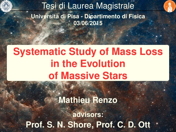
Tesi di Laurea Magistrale Universit` a di Pisa - Dipartimento di Fisica 03/06/2015 Systematic Study of Mass Loss in the Evolution of Massive Stars Mathieu Renzo advisors: Prof. S. N. Shore, Prof. C. D. Ott 1 / 27

Outline Introduction • Importance of Massive Stars • How do they lose mass? Stellar Winds • Outline of the Theory • Methods • Results: Amplitude of the Uncertainty • Results: Blue Loops in 15 M ⊙ models Impulsive Mass Loss Events • Motivations for This Study • Methods • Results: Wind + Impulsive Mass Loss • Results: pre-SN Stripped Structures Conclusions 2 / 27

Outline Introduction • Importance of Massive Stars • How do they lose mass? Stellar Winds • Outline of the Theory • Methods • Results: Amplitude of the Uncertainty • Results: Blue Loops in 15 M ⊙ models Impulsive Mass Loss Events • Motivations for This Study • Methods • Results: Wind + Impulsive Mass Loss • Results: pre-SN Stripped Structures Conclusions 3 / 27

Why are Massive Stars Important? M ZAMS � 8 − 10 M ⊙ • Nucleosynthesis • Chemical Evolution of Galaxies • Effects on Star Formation • Re-ionization Epoch • Observations of Farthest Galaxies • Catastrophic Events 4 / 27

Mass Loss – Why does it Matter... ... for the environment of the stars? • Pollution of the InterStellar Medium (ISM) • Tailoring of the CircumStellar Material (CSM) • Effects on the Star Formation ... for the stellar structure? • Evolutionary Timescales • Final Fate (BH, NS or WD?) • Light Curve and Explosion Spectrum • Appearance: CSM and Wind Features (e.g. WR) • Role in the Solution of the RSG Problem ? 5 / 27

Possible Mass Loss Mechanisms Radiative Driving ⇐ Stellar Winds Dynamical Instabilities ⇐ LBVs, Impulsive Mass Loss, Pulsations, Super-Eddington Winds Binary interactions ⇐ Roche Lobe OverFlows Figure: η Carinae. (RLOF) 6 / 27

Outline Introduction • Importance of Massive Stars • How do they lose mass? Stellar Winds • Outline of the Theory • Methods • Results: Amplitude of the Uncertainty • Results: Blue Loops in 15 M ⊙ models Impulsive Mass Loss Events • Motivations for This Study • Methods • Results: Wind + Impulsive Mass Loss • Results: pre-SN Stripped Structures Conclusions 7 / 27

Radiatively Driven Winds in One Slide ∆ p = h c ( ν i cos ( θ i ) − ν f cos ( θ f )) Problems: High Non-Linearity and Clumpiness: = � ρ 2 � def � ρ � 2 � = 1 ⇒ Inhomogeneities ⇒ ˙ M � = 4 π r 2 ρ v ( r ) f cl 8 / 27

Radiatively Driven Winds in One Slide Risk: ∆ p = h Possible Overestimation of the c ( ν i cos ( θ i ) − ν f cos ( θ f )) Wind Mass Loss Rate Problems: High Non-Linearity and Clumpiness: = � ρ 2 � def � ρ � 2 � = 1 ⇒ Inhomogeneities ⇒ ˙ M � = 4 π r 2 ρ v ( r ) f cl 8 / 27

Mass Loss in (Semi–)Empirical parametric models. Uncertainties encapsulated in efficiency factor: ˙ M ( L , T eff , Z , R , M , ... ) ⇐ η ˙ M ( L , T eff , Z , R , M , ... ) η is a free parameter: η ∈ [ 0, + ∞ ) Figure: From Smith 2014, ARA&A, 52, 487S 9 / 27

Different dM / dt algorithms with Grid of Z ⊙ ≃ 0.019 , non-rotating stellar models: • Initial mass: M ZAMS = { 15, 20, 25, 30 } M ⊙ ; • Efficiency: f cl = { 1, 1 1 � η ≡ 10 } ; 3 , • Different combinations of wind mass loss rates for “hot” ( T eff ≥ 15 [ kK ] ), “cool” ( T eff < 15 [ kK ] ) and WR stars: Kudritzki et al. ’89; Vink et al. ’00, ’01; Van Loon et al. ’05; Nieuwenhuijzen et al. ’90; De Jager et al. ’88; Nugis & Lamers ’00; Hamann et al. ’98. 10 / 27

Results: Relative Final Mass 1.0 VdJNL VdJNL VNJNL VNJNL 0.9 VNJH VNJH 0.8 VdJH VdJH M O depl / M ZAMS VvLH VvLH 0.7 VvLNL VvLNL KdJNL KdJNL 0.6 KNJNL KNJNL KNJH KNJH 0.5 KdJH KdJH 0.4 KvLH KvLH KvLNL KvLNL 0.3 15 20 25 30 M ZAMS [ M ⊙ ] Diamonds ⇔ η = 1.0 , Squares ⇔ η = 0.33 , Circles ⇔ η = 0.1 . 11 / 27

M ( t ) for M ZAMS = 15 M ⊙ with 15 14 13 12 Vink et al. , de Jager et al. Kudritzki et al. , Nieuwenhuijzen et al. 11 M [ M ⊙ ] Kudritzki et al. , de Jager et al. 10 Vink et al. , Nieuwenhuijzen et al. 9 Kudritzki et al. , van Loon et al. Vink et al. , van Loon et al. TAMS 8 η = 1.0 7 η = 0.33 M ZAMS = 15 M ⊙ η = 0.1 6 0 1 2 3 4 5 6 7 8 9 10 11 12 13 14 t [Myr] ;

M ( t ) for M ZAMS = 15 M ⊙ with 15 14 Only η = 1.0 13 12 Vink et al. , de Jager et al. Kudritzki et al. , Nieuwenhuijzen et al. 11 M [ M ⊙ ] Kudritzki et al. , de Jager et al. 10 Vink et al. , Nieuwenhuijzen et al. 9 Kudritzki et al. , van Loon et al. Vink et al. , van Loon et al. TAMS 8 η = 1.0 7 η = 0.33 M ZAMS = 15 M ⊙ η = 0.1 6 0 1 2 3 4 5 6 7 8 9 10 11 12 13 14 t [Myr] ; 12 / 27

Comparison of Hot Wind Algorithms Example: M ZAMS = 15 M ⊙ evolutionary tracks 5.2 5.2 Kudritzki et al. , de Jager et al. Vink et al. , de Jager et al. 5.1 5.1 5.0 5.0 4.9 4.9 4.8 4.8 log ( L / L ⊙ ) log ( L / L ⊙ ) 4.7 4.7 4.6 4.6 4.5 4.5 η = 1.0 η = 1.0 4.4 4.4 η = 0.33 η = 0.33 4.3 4.3 η = 0.1 η = 0.1 4.2 4.2 4.6 4.4 4.2 4.0 3.8 3.6 3.4 4.6 4.4 4.2 4.0 3.8 3.6 3.4 log ( T eff / [ K ]) log ( T eff / [ K ]) ⇒ Early (“hot”) wind influences subsequent evolution 13 / 27

Why Blue Loops? 1/2 • Blue loop ⇔ Large He-core • Convection mixes H down, determining M He • µ is higher in He-rich regions 2 15 M ⊙ , Vink et al. , T eff = 15000 K 0 0.6 − 2 − 4 0.4 0.2 η = 1.0 − 6 log 10 ( ρ / [ g cm − 3 ]) η = 0.1 − 8 0.0 η = 0.33 4.3 4.4 4.5 4.6 4.7 4.8 − 10 2 15 M ⊙ , Kudritzki et al. , T eff = 15000 K 0 − 2 0.6 0.4 − 4 0.2 η = 1.0 − 6 η = 0.1 0.0 − 8 η = 0.33 4.3 4.4 4.5 4.6 4.7 4.8 − 10 0 1 2 3 4 5 6 7 8 9 10 11 12 13 14 15 M [ M ⊙ ] 14 / 27

Why Blue Loops? 2/2 • Blue loop starts when H-burning shell reaches the edge of the He core • Lower µ and higher X ⇒ Variations of ε nuc • Envelope responds on its thermal timescale ⇐ • if η < 1 ⇒ He core edge too deep for Blue Loops • Vink et al. rate yields larger cores allowing for Blue Loops 15 / 27

Why not Blue Loops? 2 de Jager et al. Hot wind: Vink et al. , η = 1.0 van Loon et al. 0 Nieuwenhuijzen et al. log 10 ( ρ [ g cm − 1 ]) − 2 M ZAMS = 15 M ⊙ age ≃ 13.3 [Myr] − 4 − 6 ε nuc ≥ 10 4 [ erg g − 1 s − 1 ] − 8 5 6 7 8 9 10 11 12 13 14 M [ M ⊙ ] ; Density profiles at the onset of Blue Loops

Why not Blue Loops? 2 de Jager et al. Hot wind: Vink et al. , η = 1.0 van Loon et al. 0 Nieuwenhuijzen et al. log 10 ( ρ [ g cm − 1 ]) − 2 M ZAMS = 15 M ⊙ 0 age ≃ 13.3 [Myr] − 4 − 6 ε nuc ≥ 10 4 [ erg g − 1 s − 1 ] − 8 5 6 7 8 9 10 11 12 13 14 M [ M ⊙ ] ; ρ Ideal gas EOS: P gas = µ m p k b T 16 / 27

Summary Results of the Comparison of Wind Algorithms: • η has a larger influence on the final mass than the wind algorithm; • Early (“hot phase”) mass loss influences the further evolution; ˙ M is more uncertain when it is higher (RSG phase); • • Different algorithmic representations of stellar winds ⇒ Qualitatively different evolutionary tracks; • Small number (8) of WR stars, none with η < 1 ⇒ Other mass loss mechanism(s) to form WR? 17 / 27

Outline Introduction • Importance of Massive Stars • How do they lose mass? Stellar Winds • Outline of the Theory • Methods • Results: Amplitude of the Uncertainty • Results: Blue Loops in 15 M ⊙ models Impulsive Mass Loss Events • Motivations for This Study • Methods • Results: Wind + Impulsive Mass Loss • Results: pre-SN Stripped Structures Conclusions 18 / 27

Why Impulsive Mass Loss? Observational Evidence: • LBVs • Progenitors of H-poor core collapse SNe ( ∼ 30% ) • Dense CSM for Type IIn SNe Theory: Dynamical Events ⇒ not ready • Pulsational Instabilities • Roche Lobe Overflow in binaries • Catastrophic Eruption(s) ∆ M wind ≪ ∆ M impulsive (?) 19 / 27

The Stripping Process 5.2 unstripped 5.1 M = 15 M ⊙ , Z = Z ⊙ 5.0 Remove mass in steps of 1 M ⊙ , MCE 4.9 max { ∆ M impulsive } = 7 M ⊙ . log 10 ( L / L ⊙ ) 4.8 4.7 4.6 mSGB 4.5 4.4 4.3 hMR 4.2 4.5 4.4 4.3 4.2 4.1 4.0 3.9 3.8 3.7 3.6 log 10 ( T eff / [ K ]) Red dot : T eff = 10 4 [ K ] ; Yellow Triangle : R ≥ R max /2 = 375 R ⊙ ; Cyan Diamond : Maximum Extent Convective Envelope. 20 / 27

Chosen Stripping Points 5.2 unstripped 5.1 M = 15 M ⊙ , Z = Z ⊙ 5.0 MCE 4.9 log 10 ( L / L ⊙ ) 4.8 4.7 4.6 mSGB 4.5 4.4 4.3 hMR 4.2 4.5 4.4 4.3 4.2 4.1 4.0 3.9 3.8 3.7 3.6 log 10 ( T eff / [ K ]) t ( MCE ) − t ( mSGB ) ≃ 10 4 [ yr ] ≪ 14.13 × 10 6 [ yr ] 21 / 27

Stripped series on the HR diagram Evolutionary tracks depend only on ∆ M impulsive 5.2 5.0 MCE log 10 ( L / L ⊙ ) 4.8 4.6 4.4 mSGB hMR 4.2 4.4 4.2 4.0 3.8 3.6 4.4 4.2 4.0 3.8 3.6 4.4 4.2 4.0 3.8 3.6 log 10 ( T eff / [ K ]) 22 / 27

Evolution toward Higher T eff 5.2 E unstripped G 5.1 MCE 7 M ⊙ F 5.0 MCE 7 M ⊙ , η = 0 D A 4.9 log 10 ( L / L ⊙ ) 4.8 C 4.7 B 4.6 4.5 4.4 3.75 3.70 3.65 3.60 3.55 log 10 ( T eff / [ K ]) Impulsive + wind mass loss drives blueward evolution 23 / 27