System FC and type inference AFP Summer School Wouter Swierstra and - PowerPoint PPT Presentation
System FC and type inference AFP Summer School Wouter Swierstra and Alejandro Serrano Faculty of Science Information and Computing Sciences 1 System FC or GHC Core System F plus Algebraic data types and pattern matching let bindings
System FC and type inference AFP Summer School Wouter Swierstra and Alejandro Serrano Faculty of Science Information and Computing Sciences 1
System FC or GHC Core System F ω plus ▶ Algebraic data types and pattern matching ▶ let bindings as a primitive ▶ Coercions (build-in equality proofs) ▶ Promoted data types ▶ Roles (not discussed here) Faculty of Science Information and Computing Sciences 2
System F ω Your usual λ-calculus where ▶ Abstractions are annotated with the type ▶ Type abstraction and application is explicit e ::= x (variables) | e e (application) | λ (x : τ ) . e (abstraction) | e @ τ (type application) | Λ ( α : κ ) . e (type abstraction) For example, here is how we defjne and use id id = Λ ( α : *). λ (x : α ). x > id @Bool True Faculty of Science Information and Computing Sciences 3
ADTs and pattern matching e ::= ... | case e of K x1 ... xn -> e ... L y1 ... ym -> e ▶ Pattern matching is only allowed to look at one layer ▶ Complex pattern have to be turned into a case -tree ▶ Operationally, case drives evaluation Faculty of Science Information and Computing Sciences 4
Coercions – the C in FC Built-in version of Equal data type e ::= ... | e |> γ (coercion application - cast) ::= refl (reflexivity) γ | sym γ (symmetry) | γ 1 ; γ 2 (transitivity) | K γ 1 .. γ n (same constructor) | ... ::= ... τ | τ ~ τ (type equality) Faculty of Science Information and Computing Sciences 5
coerce = Λ (a : *). Λ (b : *). λ ( : a ~ b). λ (x : a). x |> Coercions – the C in FC Take the following Haskell term coerce :: a ~ b => a -> b coerce x = x How does it look like in System FC? Faculty of Science Information and Computing Sciences 6
Coercions – the C in FC Take the following Haskell term coerce :: a ~ b => a -> b coerce x = x How does it look like in System FC? coerce = Λ (a : *). Λ (b : *). λ ( γ : a ~ b). λ (x : a). x |> γ Faculty of Science Information and Computing Sciences 6
class Show a where show :: a -> String ===> data ShowDict a = ShowDict { show :: a -> String } shout :: Show a => a -> String shout x = show x ++ "!" ===> shout :: ShowDict a -> a -> String shout sd a = show sd x ++ "!" Where are type classes? Type classes are translated to records ▶ This is called the dictionary translation Faculty of Science Information and Computing Sciences 7
Where are type classes? Type classes are translated to records ▶ This is called the dictionary translation class Show a where show :: a -> String ===> data ShowDict a = ShowDict { show :: a -> String } shout :: Show a => a -> String shout x = show x ++ "!" ===> shout :: ShowDict a -> a -> String shout sd a = show sd x ++ "!" Faculty of Science Information and Computing Sciences 7
shout = Λ (a : *). λ (sd : ShowDict a). λ (x : a). (++) @Char (show @a sd x) ((:) @Char '!' ([] @Char)) Dictionary translation, arguments shout :: ShowDict a -> a -> String shout sd a = show sd x ++ "!" Try to write it as a System FC term! Faculty of Science Information and Computing Sciences 8
Dictionary translation, arguments shout :: ShowDict a -> a -> String shout sd a = show sd x ++ "!" Try to write it as a System FC term! shout = Λ (a : *). λ (sd : ShowDict a). λ (x : a). (++) @Char (show @a sd x) ((:) @Char '!' ([] @Char)) Faculty of Science Information and Computing Sciences 8
Dictionary translation, instances ▶ Simple instances are plain values boolShow :: ShowDict Bool boolShow = ShowDict $ \x -> case x of True -> "True" False -> "False" ▶ Recursive instances are functions maybeShow :: ShowDict a -> ShowDict (Maybe a) maybeShow sd = ShowDict $ \x -> case x of Nothing -> "Nothing" Just y -> "Just " ++ show sd y Faculty of Science Information and Computing Sciences 9
Dictionary translation, superclasses Superclasses appear as fjelds of the child class class Eq a => Ord a where compare :: a -> a -> Ordering ===> data OrdDict a = OrdDict { eqDict :: EqDict a, compare :: a -> a -> Ordering } Faculty of Science Information and Computing Sciences 10
The need for inference In surface Haskell many information is implicit ▶ Type abstraction and application ▶ Dictionaries for type class instances On the other hand they are explicit in System FC Inference is the process of obtaining that information Faculty of Science Information and Computing Sciences 11
Answer We cannot unless we know the types of the free variables. Types and free variables Question: How do we assign a type to a term with free variables? plus x one Faculty of Science Information and Computing Sciences 12
Types and free variables Question: How do we assign a type to a term with free variables? plus x one Answer We cannot unless we know the types of the free variables. Faculty of Science Information and Computing Sciences 12
Environments We therefore do not assign types to terms, but types to terms in a certain environment (also called context ). Environments Γ ::= ε -- empty environment | Γ , x : τ -- binding Later bindings for a variable always shadow earlier bindings. Faculty of Science Information and Computing Sciences 13
The typing relation A statement of the form Γ ⊢ e : τ means “in environment Γ , term e has type τ ”. This defjnes a ternary relation between an environment, a term and a type. The ⊢ (called turnstile) and the colon are just notation for making the relation look nice but carry no meaning. We could have chosen the notation T( Γ ,e, τ ) for the relation as well, but Γ ⊢ e : τ is commonly used. Faculty of Science Information and Computing Sciences 14
Type rules The relation is defjned inductively, using inference rules . Variables x : τ ∈ Γ Γ ⊢ x : τ ▶ Above the bar are the premises . ▶ Below the bar is the conclusion . ▶ If the premises hold, we can infer the conclusion. Faculty of Science Information and Computing Sciences 15
(Hindley-)Damas-Milner type inference Mainly based on a paper by Milner (1978). This algorithm is: ▶ the basis of the algorithm used for the ML family of languages as well as Haskell; ▶ allows type inference essentially for the simply-typed lambda calculus extended with a limited form of polymorphism (sometimes called let -polymorphism); ▶ is a “sweet spot” in the design space: some simple extensions are possible (and performed), but fundamental extensions are typically signifjcantly more diffjcult. Faculty of Science Information and Computing Sciences 16
Monotypes and type schemes Damas-Milner types are all quantifjed at the outermost level. That is why Haskell typically does not use an explicit universal quantifjer. Monotypes Monotypes τ are types built from variables and type constructors. Type schemes (or polytypes) σ ::= τ -- monotypes | ∀ α . s -- quantified type Faculty of Science Information and Computing Sciences 17
The key idea The Damas-Milner algorithm distinguishes lambda-bound and let-bound (term) variables: ▶ lambda-bound variables are always assumed to have a monotype; ▶ let-bound variables, we know what they are bound to, therefore they can have polymorphic type. Faculty of Science Information and Computing Sciences 18
Inference variables Whenever a lambda-bound variable is encountered, a fresh inference variable is introduced. The variable represents a monotype. When we learn more about the types, inference variables can be substituted by types. Inference variables are difgerent from universally quantifjed variables that express polymorphism. Faculty of Science Information and Computing Sciences 19
Term language e ::= x -- variables | e e -- application | \x -> e -- abstraction | let x = e in e -- let binding Only a simple language to start with, but we include let compared to plain lambda calculus. Faculty of Science Information and Computing Sciences 20
To typecheck neg x , we fjrst determine the types of the components. In the environment we can fjnd the types of the variables: neg : Nat -> Nat and x : v . We now unify Nat and v , introducing the substitution: Nat . v Example Assume an environment Γ = neg : Nat -> Nat . Consider inferring the type of the expression \x -> neg x . For x , we introduce an type variable v and assume x : v . Faculty of Science Information and Computing Sciences 21
In the environment we can fjnd the types of the variables: neg : Nat -> Nat and x : v . We now unify Nat and v , introducing the substitution: Nat . v Example Assume an environment Γ = neg : Nat -> Nat . Consider inferring the type of the expression \x -> neg x . For x , we introduce an type variable v and assume x : v . To typecheck neg x , we fjrst determine the types of the components. Faculty of Science Information and Computing Sciences 21
Recommend
More recommend
Explore More Topics
Stay informed with curated content and fresh updates.
