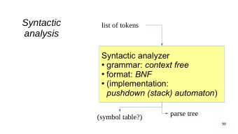
Syntactic Formalisms 2 MPRI 4 I. Context-Free Grammars 3 MPRI 4 - PowerPoint PPT Presentation

1 MPRI 4 Syntactic Formalisms

2 MPRI 4 I. Context-Free Grammars

3 MPRI 4 • Definition G = ( N, T, P, S ) where: ◦ N is a finite set of non-terminal symbols; ◦ T is a finite set of terminal symbols; ◦ P is a finite set of production rules A → α where A ∈ N and α ∈ ( N ∪ T ) ∗ ◦ S ∈ N is the start symbol. L ( G ) = { ω ∈ T ∗ | S → ∗ ω }

4 MPRI 4 Example • Grammatical rules S → NP VP VP → tV NP VP → stV Adj NP → Det N • Lexicon tV → /mange/ stV → /est/ NP → /Pierre/ N → /fruit/ Adj → /intelligent/ Det → /un/

5 MPRI 4 CKY Algorithm init <A → • α, i, i> scan <A → α • aβ, i, j> a = a j +1 <A → αa • β, i, j + 1 > complete <A → α • Bβ, i, j> <B → γ • , j, k> <A → αB • β, i, k> • Good news/Bad news

6 MPRI 4 Earley Algorithm init <S → • α, 0 , 0 > scan <A → α • aβ, i, j> a = a j +1 <A → αa • β, i, j + 1 > complete <A → α • Bβ, i, j> <B → γ • , j, k> <A → αB • β, i, k> predict <A → α • Bβ, i, j> <B → • γ, j, j> • Correct-prefix property

7 MPRI 4 II. Unification Grammars

8 MPRI 4 Suppose we extend our toy grammar with the following rules: NP → NP Conj NP Conj → /et/ NP → /Marie/ N → /pomme/ Det → /une/ Det → /des/ We get: ∗ Marie est intelligent ∗ Marie mange un pomme ∗ Pierre et Marie mange une pomme ? Pierre mange Marie

9 MPRI 4 S → NP [ X, Y ] VP [ X, Y ] VP [ X, Y ] → tV [ Y ] NP [ W, Z ] VP [ X, Y ] → stV [ Y ] Adj [ X, Y ] NP [ X, Y ] Det [ X, Y ] N [ X, Y ] → NP [m , p] → NP [m , X ] Conj NP [ Y, Z ] NP [m , p] NP [ X, Y ] Conj NP [m , Z ] → NP [f , p] → NP [f , X ] Conj NP [f , Y ] tV [s] → /mange/ N [f , p] → /pommes/ tV [p] → /mangent/ Adj [m , s] → /intelligent/ stV [s] /est/ Adj [f , s] /intelligente/ → → stV [p] → /sont/ Adj [m , p] → /intelligents/ NP [m , s] /Pierre/ Adj [f , p] /intelligentes/ → → NP [f , s] → /Marie/ Det [m , s] → /un/ N [m , s] → /fruit/ Det [f , s] → /une/ N [m , p] → /fruits/ Det [ X, p] → /des/ N [f , s] → /pomme/ Conj → /et/

10 MPRI 4 Earley Algorithm init <S → • α, 0 , 0 > scan <A → α • aβ, i, j> a = a j +1 <A → αa • β, i, j + 1 > complete <A → α • Bβ, i, j> <C → γ • , j, k> σ = mgu( B, C ) < ( A → αB • β ) σ, i, k> predict <A → α • Bβ, i, j> σ = mgu( B, C ) < ( C → • γ ) σ, j, j> • equality up to variable renaming, subsumption, completeness ?

11 MPRI 4 Carl Pollard and Ivan A. Sag: Head-Driven Phrase Structure Grammar. Uni- versity of Chicago Press, 1994. Joan Bresnan: Lexical-Functional Syntax, Oxford: Blackwell Publishers Ltd, 2001. Anne Abeill´ e: Les Nouvelles syntaxes. Armand Colin, 1993.

12 MPRI 4 III. Tree Adjoining Grammars

13 MPRI 4 • Lexicalization • Weak Equivalence versus Strong Equivalence • Definition G = ( N, T, I, A, S ) where: ◦ N is a finite set of non-terminal symbols; ◦ T is a finite set of terminal symbols; ◦ I is a finite set of trees called initial trees; ◦ A is a finite set of trees called auxiliary trees; ◦ S ∈ N is the start symbol. The trees in I ∪ A are called elementary trees. The inner nodes of the el- ementary trees are labeled by non-terminals. Their leaves are labeled by non-terminals or by terminals. In each auxiliary tree, there is one distin- guished leaf (called the foot) whose label is the same non-terminal as the label of the root.

14 MPRI 4 • Substitution S N S � � � ��������� � �������� � �������� � � � � � � � � � � � ⇒ � � � � � � � � � N N ↓ � �������� � � � initial tree � � � initial/derived tree � derived tree • Adjunction S N S � � � ��������� � ��������� � ��������� � � � � � � � � � � N N � � ⇒ � � � � � � � � � � � �������� � � � � � � � � � N ∗ � � � � N initial/derived tree � auxiliary tree � � � � � derived tree

15 MPRI 4 Example • Initial trees NP NP S � ��������� � � � � � � � � Peter Mary NP ↓ VP � �������� � � � � � � NP ↓ V kisses • Auxiliary tree VP � � ������� � � � � � � � � VP ∗ Adv possionately

16 MPRI 4 CKY Algorithm init <A → • α, i, , , i> scan <A → α • Bβ, i, j, k, l> <A → αB • β, i, j, k, l + 1 > label( B ) = a l +1 complete <A → α • Bβ, i, j, k, l> <B → γ • , l, m, n, o> <A → αB • β, i, j ⊔ m, k ⊔ n, o> i ⊔ = i ⊔ i = i undefined otherwise

17 MPRI 4 foot <A → α • Bβ, i, , , j> <A → αB • β, i, j, k, k> B is the foot of an auxiliary tree adjoin <A → α • , i, j, k, l> <B → β • , m, i, l, n> <A → β • , m, j, k, n> B is the root of an auxiliary tree label( A ) = label( B ) substitute <A → α • Bβ, i, j, k, l> <C → γ • , l, , , m> <A → αB • β, i, j, k, m> C is the root of an initial tree label( B ) = label( C )

18 MPRI 4 Example • Initial tree S e • Auxiliary tree S � � � � � � � � � � � � � � � a S d � � � � � � � � � � � � � � � � S ∗ c b • Let ω = 0 a 1 a 2 b 3 b 4 e 5 c 6 c 7 d 8 d 9

19 MPRI 4 <A 2 → • bA 3 c, 2 , , , 2 > scan <A 2 → b • A 3 c, 2 , , , 3 > foot <A 2 → • bA 3 c, 3 , , , 3 > <A 1 → • aA 2 d, 1 , , , 1 > <A 2 → bA 3 • c, 2 , 3 , 6 , 6 > scan scan scan <A 2 → b • A 3 c, 3 , , , 4 > <A 1 → a • A 2 d, 1 , , , 2 > <A 2 → bA 3 c • , 2 , 3 , 6 , 7 > foot complete <A 2 → bA 3 • c, 3 , 4 , 5 , 5 > <A 1 → aA 2 • d, 1 , 3 , 6 , 7 > scan scan <A 2 → bA 3 c • , 3 , 4 , 5 , 6 > <A 1 → aA 2 d • , 1 , 3 , 6 , 8 > adjoin <A 2 → aA 2 d • , 1 , 4 , 5 , 8 > · <A 1 → • aA 2 d, 0 , , , 0 > · scan · <A 1 → a • A 2 d, 0 , , , 1 > <A 2 → aA 2 d • , 1 , 4 , 5 , 8 > complete <A 0 → • e, 4 , , , 4 > <A 1 → aA 2 • d, 0 , 4 , 5 , 8 > scan scan <A 0 → e • , 4 , , , 5 > <A 1 → aA 2 d • , 0 , 4 , 5 , 9 > adjoin <A 0 → aA 2 d • , 0 , , , 9 >

20 MPRI 4 • Good news/Bad news • Earley algorithms (Schabes & Joshi, 1988; Schabes 1991; Nederhof 1997) • Expressive power • Adjoining constraints

21 MPRI 4 Aravind K. Joshi, K. Vijay-Shanker: Some Computational Properties of Tree Adjoining Grammars. ACL 1985: 82-93 Yves Schabes, Aravind K. Joshi: An Earley-Type Parsing Algorithm for Tree Adjoining Grammars. ACL 1988: 258-269 Yves Schabes: The valid prefix property and left to right parsing of tree- adjoining grammar. IWPT 1991: 2–30 Mark-Jan Nederhof: The Computational Complexity of the Correct-Prefix Property for TAGs. Computational Linguistics 25(3): 345-360 (1999) Eric Villemonte de la Clergerie: Tabulation et traitementde la langue na- turelle. Tutorial 1999 http://pauillac.inria.fr/˜clerger/

22 MPRI 4 IV. Range Concatenation Grammars

23 MPRI 4 • Expressive Power versus Tractability • Definition G = ( N, T, V, P, S ) where: ◦ N is a ranked alphabet of predicate names; ◦ T is a finite set of terminal symbols; ◦ V is a finite set of variable symbols; ◦ P is a finite set of clauses φ 0 → φ 1 . . . φ n where φ 0 , φ 1 . . . φ n are predicates of the form A ( α 1 , . . . , α p ) whith A ∈ N and α 1 , . . . , α n ∈ ( T ∪ V ) ∗ ; ◦ S ∈ N is the start symbol.

24 MPRI 4 • Notion of range • Given a word ω ∈ T ∗ , an instantiated clause is such that the variables and the predicate arguments are bound to ranges in ω ∈ T ∗ • Example: S ( XY ) → S ( X ) E ( X, Y ) S ( a ) → ǫ E ( Xa, Y a ) → E ( X, Y ) E ( ǫ, ǫ ) → ǫ • Complete for PTIME. • Closed by Union, Intersection, Concatenation, Iteration, Complementation.

25 MPRI 4 See papers by Pierre Boullier http://atoll.inria.fr

26 MPRI 4 V. Categorial Grammars

27 MPRI 4 • Radical approach to lexicalism • An algebra of syntactic categories • A finite set of grammatical composition rules

28 MPRI 4 A notion of syntactic category Let A be a finite set of atomic syntactic categories. The set of syntactic categories is inductively defined as follows: T A ::= A | ( T A • T A ) | ( T A \ T A ) | ( T A / T A ) Interpretation: ( α • β ) is the category of the phrases obtained by concatenating a phrase of category α with a phrase of category β . ( α \ β ) is the category of the phrases that yield a phrase of category β when appended to a phrase of category α . ( β / α ) is the category of the phrases that yield a phrase of category β when a phrase of category α is appended to them.