Sustainable Financial Obligations and Crisis Cycles Mikael Juselius - PowerPoint PPT Presentation
Sustainable Financial Obligations and Crisis Cycles Mikael Juselius and Moshe Kim 220 200 180 160 140 120 1985 1990 1995 2000 2005 2010 (a) U.S. household sector total debt to income. 10 8 6 4 2 0 2 1985 1990 1995 2000
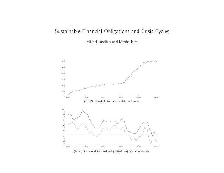
Sustainable Financial Obligations and Crisis Cycles Mikael Juselius and Moshe Kim 220 200 180 160 140 120 1985 1990 1995 2000 2005 2010 (a) U.S. household sector total debt to income. 10 8 6 4 2 0 −2 1985 1990 1995 2000 2005 2010 (b) Nominal (solid line) and real (dotted line) federal funds rate.
Outline 1. Background 2. Objectives and key findings 3. Data 4. Methodology 5. Results 6. Implications Juselius and Kim - ’Sustainable Financial Obligations and Crisis Cycles’, 3-4 November, Amsterdam 1
Background Can aggregate private sector debt reach excessive levels? • Lorenzoni (2008) and Miller and Stiglitz (2010): debt can reach (unsustainable) inefficient levels under dispersed beliefs or limited commitment in financial contracts. • King (1994) and Mian and Sufi (2010) provide cross-sectional evidence from individual episodes of financial distress suggesting close association between high aggregate leverage (debt-to-income) and subsequent credit and output losses. – They overlook the persistent upward trend that has been present in US debt to income ratios for the past 25 year, which may have been due to a concurrent decline in the real interest rate. Juselius and Kim - ’Sustainable Financial Obligations and Crisis Cycles’, 3-4 November, Amsterdam 2
– Such trends tend to have a uniform effect on the cross-section and would, hence, not generate much cross-sectional variation. • For these reasons the strong association between leverage and losses reported in cross-sectional studies, may be much weaker when viewed in a time-series context. • Borio and Lowe (2002) address the problem associated with growth trends by using leverage and asset price gaps, which are based on the Hodrick-Prescott filter. – Since this procedure is not based on economic rationale, such gaps may still confuse sustainable developments in the variables with excessive buildups. Juselius and Kim - ’Sustainable Financial Obligations and Crisis Cycles’, 3-4 November, Amsterdam 3
Objectives and key findings We model aggregate U.S. credit loss dynamics over the period 1985Q1-2010Q2, to assess the role of aggregate debt in generating both real and financial distress. We allow leverage to enter credit loss determination both linearly , in line with the literature on financial accelerators, as well as non-linearly , to capture altered be- havior and contagion effects during episodes in which aggregate credit constraints become binding (e.g., Campello et al. (2010)). Key findings : • Debt to income ratios (leverage) do not perform well as measures of excessive debt accumulations. – We find no significant temporal relationship, linear or otherwise, between aggregate leverage and credit losses. Juselius and Kim - ’Sustainable Financial Obligations and Crisis Cycles’, 3-4 November, Amsterdam 4
• An alternative measure, the financial obligations ratio (interest payments and amortizations), produce good results. – It acts as a transition variable which intensifies the interaction between credit losses and the business cycle, once a critical threshold is exceeded. – This occurs in either the household or the business sector 1-2 years prior to each economic downturn in the sample. – Together, these ratios likely play a significant role in shaping business cycle movements. Moreover, the magnitude of excessive debt in each sector seems to account for the severity and length of ensuing recessions. Juselius and Kim - ’Sustainable Financial Obligations and Crisis Cycles’, 3-4 November, Amsterdam 5
Data • We use net charge-off rates to capture credit losses. We distinguish between losses on total loans, real estate loans, and business loans. See Figure 1. • We use debt to income ratios as measures of leverage. We distinguish between the household and business sectors, and between total and real estate debt. • We use the financial obligations ratio, as constructed by the Federal Reserve, to capture interest payments and amortizations. See Figure 2. – This measure is not available for the business sector: we construct it using the federal funds rates, a fixed maturity of 3 years, and linear amortizations. • We control for several factors, such as interest rates and monetary policy. Juselius and Kim - ’Sustainable Financial Obligations and Crisis Cycles’, 3-4 November, Amsterdam 6
3.0 2.5 2.5 2.0 2.0 1.5 1.5 1.0 1.0 0.5 0.5 1985 1990 1995 2000 2005 2010 1985 1990 1995 2000 2005 2010 (a) Loss rate on total loans. (b) Loss rate on real estate loans. 3.0 2.5 2.5 2.0 2.0 1.5 1.5 1.0 1.0 0.5 0.5 1985 1990 1995 2000 2005 2010 1985 1990 1995 2000 2005 2010 (c) Loss rate on business loans. (d) Bank failure rate. 3 2 10 1 8 0 6 −1 −2 4 −3 2 −4 0 −5 1985 1990 1995 2000 2005 2010 1985 1990 1995 2000 2005 2010 (e) Output gap (f) Nominal (solid line) and real (dotted line) long-term government T- bill rate. 1.0 10 0.5 8 0.0 6 −0.5 −1.0 4 −1.5 2 −2.0 −2.5 0 −3.0 −2 −3.5 1985 1990 1995 2000 2005 2010 1985 1990 1995 2000 2005 2010 (g) Interest rate spread (h) Nominal (solid line) and real (dotted line) federal funds rate. Figure 1: Credit loss rates and various indicators of financial, monetary, and real conditions in the United Sates. The real (ex-post) interest 1 rates are constructed using the 4-quarter moving average inflation rate to facilitate the exposition.
170 220 160 200 150 140 180 130 120 160 110 100 140 90 120 80 70 1985 1990 1995 2000 2005 2010 1985 1990 1995 2000 2005 2010 (a) Total leverage in the household sector. (b) Real estate leverage in the household sector. 130 8 125 120 7 115 6 110 5 105 100 4 1985 1990 1995 2000 2005 2010 1985 1990 1995 2000 2005 2010 (c) Total leverage in the business sector. (d) Real estate leverage in the business sector. 18.5 11.0 18.0 10.5 17.5 10.0 17.0 9.5 16.5 9.0 1985 1990 1995 2000 2005 2010 1985 1990 1995 2000 2005 2010 (e) Total financial obligations in the household sector. (f) Real estate financial obligations in the household sector. 0.75 12.0 0.70 11.5 0.65 0.60 11.0 0.55 0.50 10.5 0.45 10.0 0.40 0.35 1985 1990 1995 2000 2005 2010 1985 1990 1995 2000 2005 2010 (g) Total financial obligations in the business sector. (h) Real estate financial obligations in the business sector. Figure 2: Indicators of leverage and financial obligations in the household and business sectors.
Methodology We allow the aggregate debt variables to enter credit loss determination in two ways: linearly , using a CIVAR, or nonlinearly , using a STR-model of the form: j ˜ 2 x t ) + ψ ′ d t + υ t t = (1 − ϕ ( τ t ))( µ 1 + γ ′ 1 x t ) + ϕ ( τ t )( µ 2 + γ ′ cl (1) j where ˜ cl t is the credit loss rate in loan category j , x t is a vector of explanatory variables, τ t is a transition variable, and d t is a vector of deterministic terms. The transition function takes the form ϕ ( τ t ) = 1 / (1 + e − κ 1 ( τ t − κ 2 ) ) . • The transition variable, τ t , is selected from a set which includes the leverage variables, l ij t , the financial obligations ratios, f ij t , and several control variables. • x t consists of cyclical indicators, e.g., the output gap and the term spread. Juselius and Kim - ’Sustainable Financial Obligations and Crisis Cycles’, 3-4 November, Amsterdam 7
n cl = − 0.5 * (y − y ) t t t n cl = − 0.3 * (y − y ) t t t n cl = − 0.1 * (y − y ) t t t τ t κ 2 κ 1 Figure 1: A graphical example of the regime switching STR-model. 1
Results 1. None of the debt variables are able to linearly account for credit losses and there are significant non-linearities in the data. 2. When leverage is used as τ t : the κ 2 estimate typically lie outside the variable’s range, the statistical fit is poor, and unit-roots cannot be rejected in the residuals. 3. When the financial obligations ratios are used, these problems do not occur. Juselius and Kim - ’Sustainable Financial Obligations and Crisis Cycles’, 3-4 November, Amsterdam 8
STR estimates Transition parameters Regime 1 Regime 2 cl i ˜ τ t κ 1 κ 2 γ ˜ γ ˜ γ ˜ γ ˜ iS y iS y t cl T ˜ f HR − 0 . 063 0 . 002 12 . 678 10 . 192 − 0 . 276 − 0 . 224 t t (5 . 630) (0 . 056) (0 . 045) (0 . 034) (0 . 094) (0 . 051) cl R ˜ f HR − 0 . 023 − 0 . 051 3 . 609 10 . 079 − 0 . 267 − 0 . 243 t t (1 . 128) (0 . 106) (0 . 041) (0 . 038) (0 . 099) (0 . 049) cl B ˜ f BT – – 2 . 318 10 . 44 − 0 . 249 − 0 . 619 t t (0 . 968) (0 . 199) (0 . 085) (0 . 119) Table 1: Estimated transition parameters and regime coefficients from STR-models of the credit loss rates. Recall the STR-model: ˜ 2 x t ) + ψ ′ d t + υ t cl t = (1 − ϕ ( τ t ))( µ 1 + γ ′ 1 x t ) + ϕ ( τ t )( µ 2 + γ ′ 1 ϕ ( τ t ) = 1 + e − κ 1 ( τ t − κ 2 ) . Juselius and Kim - ’Sustainable Financial Obligations and Crisis Cycles’, 3-4 November, Amsterdam 9
3 Loss rate on real estate loans Regime 1 Regime 2 2 1 0 1985 1990 1995 2000 2005 2010 Financial obligations ratio, household’s real estate debt 11 10 MSBD 9 1985 1990 1995 2000 2005 2010 Figure 1: Transitions in the loss rate on real estate loans. The upper panel depicts the loss rate on real estate loans, whereas the lower panel depicts the financial obligations ratio associated with household’s real estate debt and the corresponding MSDB estimate. Episodes when regime 2 dominate are demarked by grey bars. 1
Recommend
More recommend
Explore More Topics
Stay informed with curated content and fresh updates.
