Survival models and health sequences Walter Dempsey University of - PowerPoint PPT Presentation

Survival models and health sequences Walter Dempsey University of Michigan July 27, 2015

Problem Description Survival Data I Survival data is commonplace in medical studies, consisting of failure time information for each patient i , T i . I Many studies require patient monitoring, generating a series of measurements of a health process, Y i . A complete uncensored observation for one patient consists of the following triple: ( Y , T , t ) I Y ∼ health process (ex. CD4 cell count, Prothrombin Index, Quality of Life Index) I T ∼ failure time as measured from recruitment I t ∼ appointment schedule Joint modeling of the repeated measurements and survival data is necessary in order to gauge the e ff ect of covariates on the response. Walter Dempsey (University of Michigan) Survival models and health sequences July 27, 2015 2 / 24

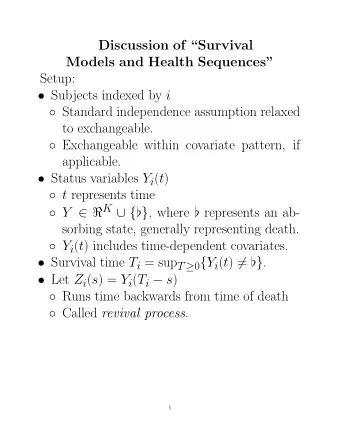
Problem Description Survival Process Survival Process A stochastic process Y i ( t ) : R ! R where R is the state space. I Typically Y i ( t ) is state of health or quality of life of patient i at time t , typically measured since recruitment I ex. Simple Survival Process, state space is R = { 0 , 1 } is su ffi cient Walter Dempsey (University of Michigan) Survival models and health sequences July 27, 2015 3 / 24

Problem Description Survival Process Survival Process A stochastic process Y i ( t ) : R ! R where R is the state space. I Typically Y i ( t ) is state of health or quality of life of patient i at time t , typically measured since recruitment I ex. Simple Survival Process, state space is R = { 0 , 1 } is su ffi cient Flatlining An absorbing state [ 2 R such that Y ( t ) = [ ) Y ( t 0 ) = [ for all t 0 > t . The survival time, T , is the time to failure: T i = sup { t : Y i ( t ) 6 = [ } Walter Dempsey (University of Michigan) Survival models and health sequences July 27, 2015 3 / 24

Problem Description Appointment Schedule The appointment schedule is a random subset t ⇢ [0 , T ), which is informative for survival regardless of health trajectory Sequential Conditional Independence Consider patient with k appointments t ( k ) = ( t 0 < . . . < t k � 1 ). The sequence Y [ t ( k ) ] may a ff ect the scheduled appointment date t k . The sequential conditional independence assumption states ? Y | ( T , t ( k ) , Y [ t ( k ) ]) . t k ? (1) (Example) Half of patients had appointment within the last three weeks of life ! unclear if assumption is violated by patient-initiated appointments (71 within 10 days prior to death). Walter Dempsey (University of Michigan) Survival models and health sequences July 27, 2015 4 / 24

Problem Description Motivating Example : Prednisone Case Study I From 1962 to 1969, 488 patients with histologically verified liver cirrhosis at hospitals in Copenhagen were randomly assigned to the two treatment arms. I 251 and 237 patients in the prednisone and placebo treatment groups respectively I 292 uncensored records ⇒ 40% patients have censored records (45% of total measurements correspond to censored patient records) I The purpose of the trial was to ascertain whether prednisone prolonged survival for patients with cirrhosis. 140 120 100 Prothrombin Index 80 60 40 20 0 0 1 2 3 4 5 Time Since Recruitment Walter Dempsey (University of Michigan) Survival models and health sequences July 27, 2015 5 / 24

Problem Description Motivating Example : Prednisone Case Study Table 1 shows average Y -values by T and t . The cell averages 8–266 non-independent, highly variable measurements. Table 1 : Average prothrombin levels indexed by T and t Survival Time t after recruitment (yrs) time ( T ) 0–1 1–2 2–3 3–4 4–5 5–6 6–7 7–8 8+ 0–1 58.0 1–2 72.5 66.4 2–3 72.6 73.2 66.0 3–4 69.8 71.2 68.5 54.2 4–5 68.5 75.7 72.5 74.6 57.7 5–6 70.5 77.3 73.5 57.1 64.5 60.9 6–7 81.8 73.6 81.1 80.6 79.4 75.5 75.8 7–8 84.4 88.8 88.1 92.1 85.2 81.2 84.3 88.1 8+ 77.3 73.6 87.0 74.1 92.0 80.3 89.2 79.4 84.7 Suggests reverse-time is a more e ff ective way of organizing the data to display main trends in the mean response. Walter Dempsey (University of Michigan) Survival models and health sequences July 27, 2015 6 / 24

Revival Process Section 2 Revival Process Walter Dempsey (University of Michigan) Survival models and health sequences July 27, 2015 7 / 24

Revival Process Revival Model The Revival Process Assuming the survival time is finite with probability one , we can define the Revival Process Z i ( s ) = Y i ( T i � s ) I The revival process is the re-aligned health process. I This is well-defined conditional on the survival time and provides an invertible mapping from the survival process to the joint survival time and revival process. Y $ ( Z , T ) I We consider this joint process in lieu of the survival process as we hope it provides e ff ective alignment of patient records for comparison and signal extraction. Walter Dempsey (University of Michigan) Survival models and health sequences July 27, 2015 8 / 24

Revival Process Revival Model The Revival Process Table 2 confirms there is considerable excess variation associated with rows (116.8) and with the reverse-time factor (77.8) but not so much with columns. Table 2 : ANOVA decomposition for Table 1 k P U Y k 2 � k P V Y k 2 Source U / V d.f. M.S. Diagonal ( R + C + D ) / ( R + C ) 544.3 7 77.8 Column ( R + C + D ) / ( R + D ) 237.9 7 34.0 Row ( R + C + D ) / ( C + D ) 817.3 7 116.8 Residual RC / ( R + C + D ) 497.2 21 23.7 ) Time reversal yields e ff ective alignment of patient records for comparison and signal extraction. Walter Dempsey (University of Michigan) Survival models and health sequences July 27, 2015 9 / 24

Revival Process Revival Model Covariates Definition (Temporal and time-evolving variable) A temporal variable x is a function defined for every t � 0. I It is a covariate if is a function on the units (entire function is determined at baseline) I Typically implies x constant, but there are exceptions (eg. patient’s age) A time-evolving variable x 0 is a temporal variable that is not a function on the units (eg. marital status, quality of life, and air quality) Every time-evolving variable is necessarily part of the response process I The joint distribution of time-evolving variables and survival time may be used to predict survival time beyond t whose status is known at times t prior to t . I Probabilistic prediction is not possible without the requisite mathematical structure of � -fields. Walter Dempsey (University of Michigan) Survival models and health sequences July 27, 2015 10 / 24

Revival Process Revival Model Treatment e ff ect: definition and estimation I For patient i , let a i ( t ) be the treatment arm scheduled for patient i at time t . I Null level required for times at and before recruitment, t  0. I Entire temporal trajectory, a i ( t ), for t � 0 is specified at baseline and determined by randomization (ie. it is a time-dependent covariate). Let ¯ a i ( s ) = a i ( T � s ) be the treatment arm expressed in revival time. I Z ? ? T | ¯ a because T is a function of ¯ a I Lack of interference (I) : the treatment assigned to one individual has no e ff ect on the response distribution for other individuals. I Lack of interference (II) : the treatment protocol at one time has no e ff ect on the response distribution at other times. Z [ s ] ? ? ¯ a | ¯ a [ s ] Walter Dempsey (University of Michigan) Survival models and health sequences July 27, 2015 11 / 24

Revival Process Revival Model Treatment e ff ect: definition and estimation Consider two patients, one in each treatment arm, a i ( t ) = ¯ a i ( T i � t ) = 1 , a j ( t ) = ¯ a j ( T j � t ) = 0 such that x i = x j . The conventional treatment definitions are � 0 � 10 ( t ) = E ( Y i ( t ) � E ( Y j ( t )) or 10 ( t ) = E ( Y i ( t ) � E ( Y j ( t ) | T i , T j > t ) Supposing the dependence on T is additive, the di ff erence of means at revival time s E ( Z i ( s ) | T ) � E ( Z j ( s ) | T ) = ⌧ 10 ( s ) + � ( T i ) � � ( T j ) contains both a treatment e ff ect and an e ff ect due to the di ff erence in survival times. Walter Dempsey (University of Michigan) Survival models and health sequences July 27, 2015 12 / 24

Survival Prediction Conditional Distribution The joint density of ( T , t ( k ) , Y [ t ( k ) ] at ( t , t ( k ) , y ) is a product of three factors Y f ( t ) ⇥ p ( t j , y j | H j , T = t ) j < k Y Y = f ( t ) ⇥ p ( y j | H j , T = t ) ⇥ p ( t j | H j , T = t ) j < k j < k f ( t ) ⇥ g k ( y ; t � t ( k ) | t ) ⇥ Y = p ( t j | H j , T = t ) , (2) j < k where f = F 0 is the survival density, and H j is the observed history ( t ( j ) , Y [ t ( j ) ]) at time t j � 1 . We assume the appointment schedule is uninformative for prediction in the sense that p ( t k | H k , T = t ) = p ( t k | H k , T = 1 ) (3) for t k � 1 < t k < t . Walter Dempsey (University of Michigan) Survival models and health sequences July 27, 2015 13 / 24

Parameter Estimation Likelihood Factorization : Survival distribution specification Re-alignment by the survival time requires the survival time to be finite with probability one. pr ( T < 1 ) = 1 Walter Dempsey (University of Michigan) Survival models and health sequences July 27, 2015 14 / 24