Structure from Motion Computer Vision CS 143, Brown James Hays - PowerPoint PPT Presentation
11/18/11 Structure from Motion Computer Vision CS 143, Brown James Hays Many slides adapted from Derek Hoiem, Lana Lazebnik, Silvio Saverese, Steve Seitz, and Martial Hebert This class: structure from motion Recap of epipolar geometry
11/18/11 Structure from Motion Computer Vision CS 143, Brown James Hays Many slides adapted from Derek Hoiem, Lana Lazebnik, Silvio Saverese, Steve Seitz, and Martial Hebert
This class: structure from motion • Recap of epipolar geometry – Depth from two views • Affine structure from motion
Recap: Epipoles • Point x in left image corresponds to epipolar line l’ in right image • Epipolar line passes through the epipole (the intersection of the cameras’ baseline with the image plane C C
Recap: Fundamental Matrix • Fundamental matrix maps from a point in one image to a line in the other • If x and x’ correspond to the same 3d point X:
Structure from motion • Given a set of corresponding points in two or more images, compute the camera parameters and the 3D point coordinates ? ? Camera 1 Camera 3 ? Camera 2 ? R 1 ,t 1 R 3 ,t 3 R 2 ,t 2 Slide credit: Noah Snavely
Structure from motion ambiguity • If we scale the entire scene by some factor k and, at the same time, scale the camera matrices by the factor of 1/ k , the projections of the scene points in the image remain exactly the same: 1 x PX P X ( k ) k It is impossible to recover the absolute scale of the scene!
How do we know the scale of image content?
Structure from motion ambiguity • If we scale the entire scene by some factor k and, at the same time, scale the camera matrices by the factor of 1/ k , the projections of the scene points in the image remain exactly the same • More generally: if we transform the scene using a transformation Q and apply the inverse transformation to the camera matrices, then the images do not change -1 x PX PQ QX
Projective structure from motion • Given: m images of n fixed 3D points • x ij = P i X j , i = 1 ,… , m, j = 1 , … , n • Problem: estimate m projection matrices P i and n 3D points X j from the mn corresponding points x ij X j x 1 j x 3 j x 2 j P 1 P 3 P 2 Slides from Lana Lazebnik
Projective structure from motion • Given: m images of n fixed 3D points • x ij = P i X j , i = 1 ,… , m, j = 1 , … , n • Problem: estimate m projection matrices P i and n 3D points X j from the mn corresponding points x ij • With no calibration info, cameras and points can only be recovered up to a 4x4 projective transformation Q : • X → QX, P → PQ -1 • We can solve for structure and motion when • 2 mn >= 11 m +3 n – 15 • For two cameras, at least 7 points are needed
Types of ambiguity A t Projective Preserves intersection and tangency 15dof T v v A t Preserves parallellism, Affine T volume ratios 12dof 0 1 s R t Similarity Preserves angles, ratios of 7dof T length 0 1 R t Euclidean Preserves angles, lengths 6dof T 0 1 • With no constraints on the camera calibration matrix or on the scene, we get a projective reconstruction • Need additional information to upgrade the reconstruction to affine, similarity, or Euclidean
Projective ambiguity A t Q p T v v -1 x PX PQ Q X P P
Projective ambiguity
Affine ambiguity A t Affine Q A T 0 1 -1 x PX PQ Q X A A
Affine ambiguity
Similarity ambiguity s R t Q s T 0 1 -1 x PX PQ Q X S S
Similarity ambiguity
Bundle adjustment • Non-linear method for refining structure and motion • Minimizing reprojection error 2 m n P X x P X E ( , ) D , ij i j i 1 j 1 X j P 1 X j x 3 j x 1 j P 3 X j P 2 X j x 2 j P 1 P 3 P 2
Photo synth Noah Snavely, Steven M. Seitz, Richard Szeliski, "Photo tourism: Exploring photo collections in 3D," SIGGRAPH 2006 http://photosynth.net/
Structure from motion • Let’s start with affine cameras (the math is easier) center at infinity
Affine structure from motion • Affine projection is a linear mapping + translation in inhomogeneous coordinates X t x a a a x 11 12 13 x AX t Y x t y a a a y 21 22 23 Z a 2 Projection of X a 1 world origin 1. We are given corresponding 2D points ( x ) in several frames 2. We want to estimate the 3D points ( X ) and the affine parameters of each camera ( A )
Affine structure from motion • Centering: subtract the centroid of the image points n n 1 1 ˆ x x x A X b A X b ij ij ik i j i i k i n n k 1 k 1 n 1 ˆ A X X A X i j k i j n k 1 • For simplicity, assume that the origin of the world coordinate system is at the centroid of the 3D points • After centering, each normalized point x ij is related to the 3D point X i by x ˆ A X ij i j
Suppose we know 3D points and affine camera parameters … then, we can compute the observed 2d positions of each point ˆ ˆ ˆ A x x x 1 11 12 1 n ˆ ˆ ˆ A x x x 2 21 22 2 n X X X 1 2 n ˆ ˆ ˆ A x x x 3D Points (3xn) m m 1 m 2 mn Camera Parameters (2mx3) 2D Image Points (2mxn)
What if we instead observe corresponding 2d image points? Can we recover the camera parameters and 3d points? cameras (2 m ) ˆ ˆ ˆ x x x A 11 12 1 n 1 ˆ ˆ ˆ ? x x x A 21 22 2 n 2 D X X X 1 2 n ˆ ˆ ˆ x x x A m 1 m 2 mn m points ( n ) What rank is the matrix of 2D points?
Factorizing the measurement matrix AX Source: M. Hebert
Factorizing the measurement matrix • Singular value decomposition of D: Source: M. Hebert
Factorizing the measurement matrix • Singular value decomposition of D: Source: M. Hebert
Factorizing the measurement matrix • Obtaining a factorization from SVD: Source: M. Hebert
Factorizing the measurement matrix • Obtaining a factorization from SVD: This decomposition minimizes |D-MS| 2 Source: M. Hebert
Affine ambiguity ~ ~ ~ S A X • The decomposition is not unique. We get the same D by using any 3 × 3 matrix C and applying the transformations A → AC, X → C -1 X • That is because we have only an affine transformation and we have not enforced any Euclidean constraints (like forcing the image axes to be perpendicular, for example) Source: M. Hebert
Eliminating the affine ambiguity • Orthographic: image axes are perpendicular and scale is 1 a 1 · a 2 = 0 x | a 1 | 2 = | a 2 | 2 = 1 a 2 X a 1 • This translates into 3 m equations in L = CC T : i = 1 , …, m T = Id , A i L A i • Solve for L • Recover C from L by Cholesky decomposition: L = CC T • Update M and S : M = MC, S = C -1 S Source: M. Hebert
Algorithm summary • Given: m images and n tracked features x ij • For each image i, c enter the feature coordinates • Construct a 2 m × n measurement matrix D : – Column j contains the projection of point j in all views – Row i contains one coordinate of the projections of all the n points in image i • Factorize D : – Compute SVD: D = U W V T – Create U 3 by taking the first 3 columns of U – Create V 3 by taking the first 3 columns of V – Create W 3 by taking the upper left 3 × 3 block of W • Create the motion (affine) and shape (3D) matrices: ½ and X = W 3 ½ V 3 T A = U 3 W 3 • Eliminate affine ambiguity Source: M. Hebert
Dealing with missing data • So far, we have assumed that all points are visible in all views • In reality, the measurement matrix typically looks something like this: cameras points One solution: – solve using a dense submatrix of visible points – Iteratively add new cameras
A nice short explanation • Class notes from Lischinksi and Gruber http://www.cs.huji.ac.il/~csip/sfm.pdf
Recommend
More recommend
Explore More Topics
Stay informed with curated content and fresh updates.
