Strong fluctuations and cycling in biological systems Timothy Newman - - PowerPoint PPT Presentation

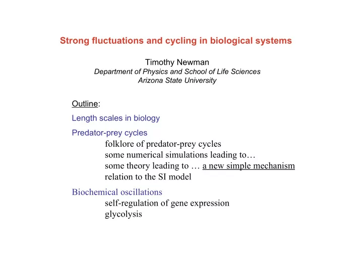
Strong fluctuations and cycling in biological systems

Timothy Newman

Department of Physics and School of Life Sciences Arizona State University

Outline: Length scales in biology Predator-prey cycles

folklore of predator-prey cycles some numerical simulations leading to… some theory leading to … a new simple mechanism relation to the SI model Biochemical oscillations self-regulation of gene expression glycolysis

Strong fluctuations in extinction and population cycles

Collaborators: Alan McKane, Physics, University of Manchester John Nagy, Biology, Scottsdale Community College Former Graduate Students: Erik DeSimone, Plant Biology, University of Cambridge Marianne Stefanini, Biomedical Engineering, Johns Hopkins University Undergraduate Students: Jeffrey Ammon, Physics, ASU Funding: Environmental Biology, NSF Mathematical Sciences, NSF NIGMS, NIH

Relevant publications

Predator-prey cycles from resonant amplification of demographic stochasticity

• A. J. McKane and T. J. Newman, Physical Review Letters 94, 218102 (2005).

Amplified biochemical oscillations in cellular systems

• A. J. McKane, J. D. Nagy, T. J. Newman, and M. O. Stefanini,

Journal of Statistical Physics, to appear October 2007 (published JSP online)

DNA/genes Proteins complexes/ reaction networks Cells Cellular aggregates Organisms Populations Ecosystems Life on earth

9

10

5

10

1

10

3

10

7

10

Information feedback Molecular biology Bio- chemistry Cell biology Develop- mental biology/ genetics Physiology Ecology and population genetics Ecosystem biology Evolution theory (adaptation/ speciation)

metres

7

10

Length scales in biology

Textbook description of cycles using population-based models (PBM)

Lotka-Volterra system V – prey density P – predator density Neutral cycles which depend on initial conditions – thus not biologically robust + logistic growth of prey Cycles disappear – replaced by damped oscillations to constant steady-state + predator satiation (non-linear functional response) Cycles reappear – as “limit cycles” Bottom line: predator satiation (or handling time) is “responsible for cycles”

' ' V rV V bPV P b PV P µ µ =

• =
• &

& (1 ) ' ' V rV V V bPV P b PV P

• µ

µ =

• =
• &

& (1 ) /(1 ) ' /(1 ) ' V rV V V bPV V P b PV V P

• µ
• µ

=

• +

= +

• &

&

But cycles are so much more intuitive than this! What’s missing?

Other mechanisms for cycling

e.g. environmental forcing, spatial coupling, new nonlinear interactions Nisbet and Gurney (1982), Aparicio and Solari (2001), Bjornstad and Grenfell (2001), Pascual, Mazzega, and Levin (2001)

An individual-based model (IBM)

It’s hard to think clearly in terms of continuous densities – let’s go back to a more fundamental description in terms of individuals: Three types of “objects”: prey (V), predators (P), and empty spaces (E) Constraint: total number of objects is fixed at N Interactions: prey birth V + E → V + V prey death V → E (not due to predation) predation P + V → P + E or P + V → P + P predator death P → E Implement as a stochastic process on a computer … and compare with mean- field theory – which is the LV equation with logistic prey reproduction

Simulation results from the IBM

Blue – solution of LV equation, Purple – average over replicates Red – one single replicate (N=3200) f1=P – number density of predators, f2=V – number density of prey

Observations are striking, but not new

The observation of large cycles in IBMs of predator-prey (or host-pathogen) systems has been previously reported – the authors were perplexed, since the IBM should behave, for large populations, in accordance with the PBM. e.g. Renshaw (1991), Rai and Singh (2000) Bartlett (1960) commented on the possibility that noise could induce cycles in disease models (SIR), but did not uncover the mechanism.

Fluctuations about the steady-stated are amplified (or resonated)

We construct a mathematical description of the system using the language of master equations. The fundamental object is Q(m,n,t) – the probability that at time t there are m prey and n predators. From the master equation one can derive mean-field equations of motion for the average number densities of predators and prey – these are identical to the LV equations. One can then take fluctuations into account for large N by expanding around mean field theory via ↔ van Kampen expansion (for large N the fluctuations will have an amplitude of 1/√ N). Naively, these fluctuations will be negligible for large N – but they’re not! The equations for x and y have the form where a, b, c, d and the noise terms are known functions of the death/birth/predation rates. (note – noise terms are correlated) Eliminating y we find an equation for x of the form This is exactly analogous to a damped pendulum with a random forcing – the pendulum will oscillate at (almost) natural frequency ω0 , since the noise has a flat frequency spectrum – i.e. the noise will automatically resonate the pendulum.

Oscillation amplitude scales as R/√N , where R is resonant enhancement at ω0 / / n N P y N = +

/ / , m N V x N = +

noise noise x ax by y cx dy = + + = + + & &

2

noise x x x

• +

+ = && &

(cf – Chubynsky’s Moscow-Kiev Bus paradigm).

Power spectra The power spectrum shows a resonant peak at a frequency equal to the cycle frequency. Blue line – theory, red line – simulation

predators prey

R ~ 30

Results directly map to SI disease dynamics

The Volterra predator-prey model is essentially identical to the classic SI model of disease dynamics, and so all of our results carry across: Three types of “objects”: susceptibles (S), infecteds (I), and empty spaces (E) Constraint: total number of objects is fixed at N Interactions: susceptible birth S + E → S + S susceptible death S → E (not due to infection) infection I + S → I + I infected death I → E These interaction rules are identical to the simplest predator-prey system: prey ↔ susceptible, predator ↔ infected

Some details on the mathematics

[ ]

'

( , ) ( | ') ( ', ) ( '| ) ( , ) dP t W P t W P t dt =

• n

n n n n n n n

, ( , ) ( , )

i i i

n N N x P t t

• =

+ = n x

1 , , 2 t i j i j i j i j

x A B = +

• ( )

i i

d F dt =

• ( )

( )

SS i i i

t t

• =

+

d

• = A
• ,

i i j j i

x A x

• =

+ &

,

( ) ( ') ( ')

i i i j

t t B t t

• =
• 2

( ) | ( ) |

i i

P x

• =

%

van Kampen expansion zeroth order first order Interested in cases where eigenvalues

• f A are complex with negative real parts
• i.e. damped transient oscillations

FP → SDE solve exactly for power spectra etc

Biochemical oscillations

The mean field equations (i.e. chemical rate equations) for each of these reaction networks have no sustained cycling behavior for any combination

• f parameter values – they are “thoroughly boring.”

Self regulation

• f gene

expression Key step in glycolysis

Calculational strategy

“Bath model” representation of reactions

M – mRNA P – protein S1 – ATP S2 – ADP A – PFK/ADP B – PFK/ADP/ATP

mRNA-protein feedback

N ~ 20,000

mRNA-protein feedback

λ=100 λ=10 ±1/√N Explicit demonstration of amplified size of oscillations

mRNA-protein feedback

Power spectrum for mRNA concentration – theory and simulation

Selkov’s model of glycolysis

N ~ 4,000 R ~ 150

Summary

We have presented a new mechanism for oscillations in populations of small to intermediate size. The essential criterion is that the mean-field (or infinite population) dynamics exhibit damped oscillations (at a frequency ω0). In a finite population, stochastic events, such as birth, death, or infection, in the form of white internal noise will automatically resonate the system at the frequency ω0 and produce large sustained oscillations. The amplitude of the oscillations scales as R / √N R – enhanced resonance factor (exactly calculable using vK expansion) N – number of individual “agents” in population We have discussed this mechanism in the context of predator-prey systems the closely related SI disease system biochemical oscillations (self-regulation of gene expression, and glycolysis) This mechanism is very general there are many further applications in biology, and other areas

Is this effect known or named?

“Stochastic resonance” would be a perfect name for this effect, but this term is already in wide-spread use for a different effect: external periodic signal applied to a non-linear system, and then a resonant periodic output being obtained using optimized noise level The term “coherence resonance” was introduced in the late ’90’s to describe i) periodic output of an excitable system in the subcritical region of a Hopf bifurcation, which is induced by internal noise ii) noise-enhanced temporal periodicity of a bursting signal the term has also attracted more widespread usage the term “self-induced stochastic resonance” has also been used to describe similar phenomena The effect described here occurs in systems which have no bifurcation points. These systems are “boring” from a deterministic viewpoint, as they have no sustained oscillatory behavior throughout their parameter space. The mechanism for noise-induced oscillations is extremely simple and can be analyzed exactly using the van Kampen expansion.