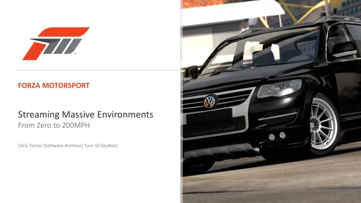
Streaming Massive Environments From Zero to 200MPH Chris Tector - PowerPoint PPT Presentation

FORZA MOTORSPORT Streaming Massive Environments From Zero to 200MPH Chris Tector (Software Architect Turn 10 Studios)

Turn 10 • Internal studio at Microsoft Game Studios - we make Forza Motorsport • Around 70 full time staff Streaming Massive Environments 2

Why am I here? • Our goals at Turn 10 • The massive model visualization hierarchy • Our pipeline, from preprocessing to the runtime Streaming Massive Environments 3

Why are you here? • Learn about streaming • Typical features in a system capable of streaming massive environments • Understand the importance of optimization in processing streaming content • Practical takeaways for your game • Primarily presented as a general system • But there are some 360 specific features which are pointed out as they are encountered Streaming Massive Environments 4

At Turn 10 GOALS Streaming Massive Environments 5

Streaming • Rendering at 60fps • Track, 8 cars and UI • Post processing, reflections, shadows • Particles, skids, crowds • Split-screen, replays Streaming Massive Environments 6

Massive Environments • Over 100 tracks, some up to 13 miles long • Over 47000 models and over 60000 textures Streaming Massive Environments 7

Zero • Looks great when standing still • All detail in there when in game or photo mode • Especially the track since it is the majority of the screen Streaming Massive Environments 8

200 • Looks great at high speeds • All detail is there when in game or replay mode, UGC video • Again, especially the track Streaming Massive Environments 9

Running Example • Le Mans is an 8.4 mile long track • It has roughly 6000 models and 3000 textures • As this talk goes on we can track how much data is streamed • Data streamed : • 13.3 Miles driven • 1.6 Laps • 0.98 GB Loaded • 0.14 GB Mesh • 0.84 GB Texture Streaming Massive Environments 10

Factors to Optimize for • Minimize • Size on disk (especially when shipping large amounts of content) • Size in memory • Maximize • Disk to memory rate • Memory to processor rate • All while maximizing quality Streaming Massive Environments 11

The Hierarchy MASSIVE MODEL VISUALIZATION Streaming Massive Environments 12

Massive Model Visualization in Research • Most relevant area to search • Good course notes from Siggraph 2007 • http://www.siggraph.org/s2007/attendees/courses/4.html • But a lot of “real time” options in the literature aren’t game real time Streaming Massive Environments 13

Typical massive model visualization hierarchy GPU/GPU Speed GPU/CPU Caches Decompressed Heap Space Compressed Cache Disk/Local Storage Streaming Massive Environments 14

Disk • Stored on zip disk in packages GPU/GPU • We store some extra data in zip format, but honor base format so standard browsing tools GPU/CPU Caches all still work (explorer, WinZip, etc.) Decompressed Heap • Stored in LZX format inside the archive Compressed Cache • 90-300MB per track Disk/Local Storage Streaming Massive Environments 15

Disk to Compressed Cache • Fast IO in cache block sizes GPU/GPU • Block is a group of files within the zip • Total up size of files until block size is reached GPU/CPU Caches • Retrieve that file group with a single read Decompressed Heap • Compressed cache reduces seeks Compressed Cache • 15MB/s peak • 10MB/s average Disk/Local Storage • But 100ms seeks Streaming Massive Environments 16

Compressed Cache • LZX format in-memory storage GPU/GPU • Cache blocks streamed in on demand and out LRU GPU/CPU Caches • 56 MB Decompressed Heap • Block sizes tuned per track, but typically 1 MB Compressed Cache Disk/Local Storage Streaming Massive Environments 17

Compressed Cache to Heaps • Fast platform specific decompression GPU/GPU • 20 MB/s average GPU/CPU Caches • Heap implementation Decompressed Heap • Optimized for speed of alloc and free operations Compressed Cache • Good fragmentation characteristics using address ordered first-fit Disk/Local Storage Streaming Massive Environments 18

Decompressed Heap • Ready for GPU or CPU to consume GPU/GPU • Contiguous and aligned per allocation GPU/CPU Caches • 194MB Decompressed Heap Compressed Cache Disk/Local Storage Streaming Massive Environments 19

Multiple Levels of Texture Storage • Three views of each texture GPU/GPU • Top Mip: Mip 0, the full resolution texture GPU/CPU Caches • Mip – Chain: Mip 1 down to 1x1 Decompressed Heap • Small Texture: 32x32 down to 1x1 Compressed Cache • Platform specific support here to not require relocating textures as top mip is streamed in Disk/Local Storage Streaming Massive Environments 20

Multiple Levels of Geometry Storage • LOD GPU/GPU • We consider different LODs as different objects to allow streaming to dump higher GPU/CPU Caches LODs when they wouldn’t contribute Decompressed Heap • Instances Compressed Cache • Models are instanced with per instance transform and shader data Disk/Local Storage Streaming Massive Environments 21

Memory to GPU/CPU Cache • CPU specific optimizations for cache friendly GPU/GPU rendering • High frequency operations have flat, cache GPU/CPU Caches line sized structures • L1/L2 Caches for CPU Decompressed Heap • Heavy use of command buffers to avoid touching Compressed Cache unnecessary render data Disk/Local Storage Streaming Massive Environments 22

GPU/CPU Caches • Right sizing of formats relative to shader needs GPU/GPU • Vertex/texture fetch caches for GPU GPU/CPU Caches • Vertex formats, stream counts • Texture formats, sizes, mip usage Decompressed Heap • Use of platform specific render controls to reduce Compressed Cache mip access, etc. Disk/Local Storage Streaming Massive Environments 23

Running Example • Data streamed : • 66.8 Miles driven • 7.9 Laps • 4.9 GB Loaded • 0.7 GB Mesh • 4.2 GB Texture Streaming Massive Environments 24

The Pipeline BREAK IT DOWN Streaming Massive Environments 25

Pre-Computed Visibility • Standard Solution • Given a scene what is actually visible at a given location • Many implementations use conservative occlusion • Our Variant Includes • Occlusion (depth buffer rejection) • LOD selection • Contribution Rejection (Don’t draw model if less than n pixels) Streaming Massive Environments 26

Culling – Given this View • Occlusion culled (square) • Other objects block this in the view • Contribution culled (circle) • This object does not contribute enough to the view Streaming Massive Environments 27

Could do it at Runtime • LOD and contribution are easy, occlusion can be implemented • Most importantly would have to optimize in runtime • Or not do it at all, but that means streaming and rendering too much • Visibility information is typically a large amount of data • Which means touching a large amount of data • Which is bad for cache performance • Our solution: don’t spend CPU/GPU on an essentially offline process Streaming Massive Environments 28

Pipeline • Our track processing pipeline is broken into 5 SAMPLING major steps • Sampling • Splitting SPLITTING • Building • Optimization BUILDING • Runtime OPTIMIZATION • All of this is fully automated • Art checks in source scenes RUNTIME • Pipeline produces optimized game ready tracks Streaming Massive Environments 29

Linearize the Space • Track is broken up into zones using AI linear view SAMPLING of track • Art generates inner and outer splines for track SPLITTING • Tools fit a central spline and normalize the BUILDING space • Waypoints are generated at regular intervals OPTIMIZATION along the central spline • Zone boundaries are set every n waypoints • Runtime Sample points are evenly distributed RUNTIME within the zones Streaming Massive Environments 30

Track Space • Track • Waypoint • Zone • Sample Streaming Massive Environments 31

How do we Sample • Environment is sampled along track surface only SAMPLING and at a limited height • Track is rendered from four views at each sample SPLITTING point • Oriented to local track space BUILDING • Sampled values stored at each sample point OPTIMIZATION • Also stored at neighboring sample points • This is to reduce visibility pops when moving RUNTIME between samples Streaming Massive Environments 32

Sampling • Render all models to depth SAMPLING • Run using position only mesh version of each model on entire track SPLITTING • Render each individual model inside a D3D BUILDING occlusion query and store • Object ID • Location of the camera during rendering OPTIMIZATION • Pixel count RUNTIME • This includes LOD, occlusion and contribution culling Streaming Massive Environments 33

Size Reduction • Sample data is enormous • Contains visibility of every model at every sample point SAMPLING • Combine all samples to reduce data required for further SPLITTING processing • We condense it down to a list of visibility of models for each BUILDING zone • Keep track of the per model maximum pixel counts, not just OPTIMIZATION binary visibility • The pixel counts are the real value! RUNTIME • Most data is used during pre-processing and then thrown out or drastically reduced for the runtime Streaming Massive Environments 34