Str Stress ess Testing Testing Cre Credit dit Risk: Risk: The - PowerPoint PPT Presentation

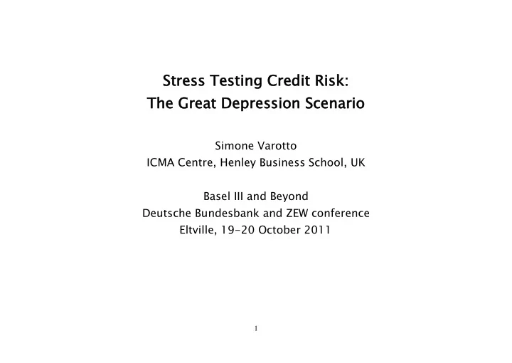
Str Stress ess Testing Testing Cre Credit dit Risk: Risk: The The Great Great Depr Depression ession Scenario Scenario Simone Varotto ICMA Centre, Henley Business School, UK Basel III and Beyond Deutsche Bundesbank and ZEW conference Eltville, 19-20 October 2011 1

Introduction  Subprime crisis and mispricing of risk o “…risk premiums were too low and long -term volatility reflected a false belief that future short-term volatility would stay at its current low levels” (Acharya et al 2009)  Stress test scenarios should be extreme but plausible o Haldane (2009) shows that plausibility may be the result of very long observation periods  Short histories are sometimes preferred to avoid structural breaks o But, crises are structural breaks!  Data limitations curtail the usefulness of historical stress testing o However, historical default rates for corporate bonds and loans available since 1920 2

 Limitations of stress tests employed by banks before the subprime crisis (Basel Committee on Banking Supervision, 2009): o Low severity and short lived scenarios compared with magnitude and time persistence of the crisis. o Correlation across and within asset classes was underestimated. o System-wide interactions (i.e. systemic risk) and feedback effects largely ignored. o Scenarios that were considered extreme and innovative were often regarded as implausible by the board and senior management 3

 Why the Great Depression? o Addresses limitations of stress tests during the recent crisis  High severity and long lived scenarios  Correlation and feedback effects embedded in historical PDs o We have been there before  Psychological explanation: if things go really bad how bad can they go? o Great Depression scenario used in the industry  In October 2008, Mark Tucker, chief executive of Prudential, stated that the Great Depression is one of the stress scenarios Prudential consider in order to test the resilience of their capital position 4

o Similarities of recent crisis with Great Depression (Eichengreen and O‟Rourke 2009) 5

o Moody‟s historical speculative grade default rates Year Sorted Default Rates (from highest) 1933 15.4 2009 13.0 1932 10.8 2001 10.3 1990 10.0 6

 Contributions of the paper o The paper tackles the question of how much capital banks should hold to be able to absorb credit losses in a Great Depression (GD) scenario. o Default and migration risk taken into account o Measured impact of extended holding periods, up to 3 years o Comparison of our results with Basel II and Basel III bank capital regulation for the banking book o Explored counter-cyclical capital buffers generated through GD stress tests 7

 Recent Literature o Carey (2002) looks at the Great Depression scenario. Focus on pre-Basel II regulation. Default mode only. o Stress testing by using macroeconomic models of credit risk: Pesaran, Schuermann, Treutler and Weiner (2006), Jokivuolle, Virolainen, Vahamaa (2008) and Huang, Zhou and Zhu (2009), among others. For an excellent survey of macro credit risk models adopted by several national regulators and central banks see Foglia (2008). o Limitations of the above models: Alfaro and Drehmann (2009) 8

o Stress testing and regulation:  Basel Committee (2006, 2009 various),  Committee of European Banking Supervisors (2009),  Financial Services Authority (2009)  IMF and World Bank‟s Financial Sector Assessment Programs (1999 to date) o Giesecke, Longstaff, Schaefer and Strebulaev (2009) study the properties of corporate bond default rates using a new data set covering the 1866−2008 period. They conclude that “in coming to grips with the current financial market sit uation which has been termed a „ historic crisis ‟ or „ the worst financial crisis since the Great Depression, ‟ nothing is so valuable as actually having a long-term historical perspective. ” 9

 Relevance: 2009 IMF Estimated Bank Portfolio Composition by Type of Asset US UK Europe Asian Banks Banks w/out UK Banks* Loan Exposures Consumer 17 12 13 20 Residential mortgage 52 23 25 26 Commercial mortgage 6 6 5 5 Corporate 15 49 43 27 Other 11 10 14 22 Total 100 100 100 100 * Asian banks domiciled in Australia, Hong Kong SAR, Japan, New Zealand and Singapore 10

The model:  Objective: to measure the amount of capital needed to absorb worst- case default losses. Worst case capital is computed from corporate default and rating migration histories going back to 1921.  We define worst-case capital as, Worst case credit loss – Expected credit loss  We measure worst case and expected losses for a buy-and-hold investor over a period of up to 3 years 11

Why should we use the buy-and-hold paradigm?  "For bank loan portfolios, substantial rebalancing [to a safer portfolio] is usually difficult to accomplish quickly, especially during the periods of general economic distress" (Carey 2002)  “… several years frequently elapse between the onset of distress [due to large credit losses] and recapitalizatio n” (Barakova and Carey 2002)  Drawing from the Japanese experience during the “ lost decade ” Caballero et al (2008) conclude that banks tend not to write off non- performing loans in a crisis, o To avoid breaching minimum capital requirements o To prevent criticism from the public and the media o Owing to political pressure to keep lending channels open (especially to SMEs) 12

 The implication of a buy and hold paradigm is that risk premia become irrelevant and we can determine credit losses under risk neutrality with physical default probabilities (Elton et al 2001, JF). This is because the buy and hold investor is not expected to liquidate his assets before expiry and hence will not face the cost of discounting them at prevailing market rates. o Then, the only relevant risk is whether a borrower defaults or not. 13

 The value of a credit exposure at a given time  can be computed with the following iterative equation,     aP C V P    t t t 1    τ τ , 1 1 , 1 V for t n         t , 1 ,..., 1 f  t 1 , 1 where C is the interest charge, n the time to maturity in years, a is the recovery rate, P τ is the (physical) probability of default in period t t ,  1 conditional on no bankruptcy in the  to t period, is the one-year f , 1 t zero-coupon risk free forward rate at time t.  The conditional default probability P τ are given by t ,  1 CP CP  t t  τ τ , , 1 P  t  τ , 1 CP  1 t  τ , 1 where CP , τ is the cumulative default probability from  to t and is t obtained through the product of annual rating transition matrices under the heterogeneous markov chain assumption. 14

 We define the default loss for a buy and hold investor as, G V  t t L  t G t Where V denotes the hold to maturity value of a corporate exposure and G is the hold to maturity value of a default risk free exposure with the same cash flows as V.  We define worst case (W) and average (A) default loss for a corporate exposure with given rating and maturity as follows,   L Max L a a   W t W t   L Average L a a   A t A t Where W a and A a are the worst case and average recovery rate respectively. Then, worst case capital is L L . Maximum and average  W A losses are computed over the whole sample period, 1921-2009. 15

Data  Moody‟s bond and loan default and transition rates by rating for the period 1921-2009 Varying "M rying "Mob obility" o " of f Ra Rating T g Tran ransit sition on M Matrices ces Ov Over er T Time Average Great Recession Great Depression Worst Case 1921-2009 2008-2009 1931-1935 1932 No Default No Default No Default No Default Migration Rate Migration Rate Migration Rate Migration Rate Aaa 92.3 0.00 76.2 0.00 82.7 0.00 67.7 0.00 Aa 91.7 0.07 81.1 0.28 80.2 0.29 53.5 0.69 A 91.4 0.10 89.1 0.28 77.3 0.67 56.0 0.92 Baa 89.5 0.28 91.7 0.65 75.3 1.34 53.3 0.94 Ba 86.5 1.14 79.0 1.86 69.6 5.87 50.2 6.33 B 85.6 3.64 76.3 4.87 68.2 10.27 54.4 15.21 Caa-C 78.1 14.67 69.0 25.78 67.9 24.15 68.4 26.32 Mobility 11.7 21.0 25.5 44.5 16

Min inim imum um an and Ave d Average rage Rec Recove overy Rate ry Rates f for Bank Loans r Bank Loans Paper Minimum Average Notes Recovery (%) Recovery (%) Araten et al. JPMorgan Chase data, 1982- 46.50 63.06 (2004) 1999 sample. Asarnow et Citigroup data, 1970-1993 52.39 66.04 al. (1995) sample. Emery 50.00 65.00 Moody's estimates (2008) Felsovalyi et Citibank data, 1970-1996 53.40 69.66 al. (1998) sample. 17

Wo Worst C rst Case se C Capi pita tal based sed on on th the Gr Great D t Dep epre ress ssion on S Scena cenario Portfo ortfolio C o Cre redit t Qua Quality ty High Average Low Very Low Holding Period (yrs) Default Risk Only 1 1.69 3.32 5.48 5.99 2 2.63 5.16 8.75 9.65 3 3.14 6.18 10.56 11.76 Default and Migration Risk 1 1.69 3.32 5.48 5.99 2 4.07 6.60 10.14 10.99 3 5.27 8.34 12.58 13.69 18