Stoichiometric network analysis In stoichiometric analysis of - PowerPoint PPT Presentation
Stoichiometric network analysis In stoichiometric analysis of metabolic networks, one concerns the effect of the network structure on the behaviour and capabilities of metabolism. Questions that can be tackled include: Discovery of pathways
Stoichiometric network analysis In stoichiometric analysis of metabolic networks, one concerns the effect of the network structure on the behaviour and capabilities of metabolism. Questions that can be tackled include: ◮ Discovery of pathways that carry a distinct biological function (e.g. glycolysis) from the network, discovery of dead ends and futile cycles, dependent subsets of enzymes ◮ Identification of optimal and suboptimal operating conditions for an organism ◮ Analysis of network flexibility and robustness, e.g. under gene knockouts
Stoichiometric coefficients Soitchiometric coefficients denote the proportion of substrate and product molecules involved in a reaction. For example, for a reaction r : A + B �→ 2 C , the stoichiometric coefficients for A , B and C are − 1 , − 1 and 2, respectively. ◮ Assignment of the coeefficients is not unique: we could as well choose − 1 / 2 , − 1 / 2 , 1 as the coefficients ◮ However, the relative sizes of the coeefficients remain in any valid choice. ◮ Note! We will denote both the name of a metabolite and its concentration by the same symbol.
Reaction rate and concentration vectors ◮ Let us assume that our metabolic network has the reactions R = { R 1 , R 2 , . . . , R r } ◮ Let the reaction R i operate with rate v i ◮ We collect the individual reaction rates to a rate vector v = ( v 1 , . . . , v r ) T ◮ Similarly, the concentration vector X ( t ) = ( X 1 ( t ) , . . . , X m ( t )) T contains the concentration of each metabolite in the system (at time t )
Stoichiometric vector and matrix ◮ The stoichiometric · 0 coefficients of a reaction · 0 are collected to a vector s r A − 1 ◮ In s r there is a one position · 0 for each metabolite in the s r = · 0 metabolic system − 1 B ◮ The stoichiometric · 0 co-efficient of the reaction · 0 are inserted to appropriate 2 C positions, e.g. for the reaction r : A + B �→ 2 C ,
Stoichiometric matrix ◮ The stoichiometric vectors stoichiometric coeefficients can be combined into the of of the reaction j . stoichiometric matrix S . ◮ In the matrix S , the is one row for each metabolite s 11 · · · s 1 j · · · s 1 r M 1 , dots , M m and one . . . ... ... . . . . . . column for each reaction · · · · · · S = s i 1 s ij s ir R 1 , . . . , R r . . . . ... ... . . . ◮ The coefficients s ∗ j along . . . the j ’th column are the s m 1 · · · s mj · · · s mr
Systems equations In a network of m metabolites and r reactions, the dynamics of the system are characterized by the systems equations r dX i � dt = s ij v j , for i = 1 , . . . , m j =1 ◮ X i is the concentration of the i th metabolite ◮ v j is the rate of the j th reaction and ◮ s ij is the stoichiometric coefficient of i th metabolite in the j th reaction. Intuitively, each system equation states that the rate of change of concentration of a is the sum of metabolite flows to and from the metabolite.
Systems equations in matrix form ◮ The systems equation can be expressed in vector form as r dX i � s ij v j = S T dt = i v , j =1 where S i contains the stoichiometric coefficients of a single metabolite, that is a row of the stoichiometric matrix ◮ All the systems equations of different equations together can then be expressed by a matrix equation d X dt = S v , ◮ Above, the vector � T d X � d X 1 dt , . . . , d X n dt = dt collects the rates of concentration changes of all metabolites
Steady state analysis ◮ Most applications of stoichiometric matrix assume that the system is in so called steady state ◮ In a steady state, the concentrations of metabolites remain constant over time, thus the derivative of the concentration is zero: r dX i � dt = s ij v j = 0 , for i = 1 , . . . , n j =1 ◮ The requires the production to equal consumption of each metabolite, which forces the reaction rates to be invariant over time.
Steady state analysis and fluxes ◮ The steady-state reaction rates v j , j = 1 , . . . , r are called the fluxes ◮ Note: Biologically, live cells do not exhibit true steady states (unless they are dead) ◮ In suitable conditions (e.g. continuous bioreactor cultivations) steady-state can be satisfied approximately. ◮ Pseudo-steady state or quasi-steady state are formally correct terms, but rarely used r dX i � dt = s ij v j = 0 , for i = 1 , . . . , n j =1
Defining the system boundary When analysing a metabolic system we need to consider what to include in our system We have the following choices: 1. Metabolites and reactions internal to the cell (leftmost picture) 2. (1) + exchange reactions transporting matter accross the cell membrane (middle picture) 3. (1) + (2) + Metabolites outside the cell (rightmost picture) (Picture from Palsson: Systems Biology, 2006)
System boundary and the total stoichiometric matrix The placement of the system boundary reflects in the � S II � S IE S = stoichiometric matrix that will 0 S EE partition into four blocks: ◮ S II : contains the stoichiometric coefficients of internal metabolites w.r.t internal reactions ◮ S IE : coefficients of internal metabolites in exchange reactions i.e. reactions transporting metabolites accross the system boundary ◮ S EI (= 0) : coefficients of external metabolites w.r.t internal reactions; always identically zero ◮ S EE : coefficients of external metabolites w.r.t exchange reactions; this is a diagonal matrix.
Exchange stoichiometrix matrix In most applications handled on this course we will not consider external compounds ◮ The (exchange) stoichiometric matrix, containing the internal metabolites and both internal and exchange reactions, will be used � � S = S II S IE ◮ Our metabolic system will be then open, containing exhange reactions of type A ⇒ , and ⇒ B
System boundary and steady state analysis ◮ Exchange stoichiometric matrix is used for steady state analysis for a reason: it will not force the external metabolites to satisfy the steady state condition r dX i � dt = s ij v j = 0 , for i = 1 , . . . , n j =1 ◮ Requiring steady state for external metabolites would drive the rates of exchange reactions to zero ◮ That is, in steady-state, no transport of substrates into the system or out of the system would be possible!
Internal stoichiometrix matrix ◮ The internal stoichiometric matrix, containing only the internal metabolites and internal reactions can be used for analysis of conserved pools in the metabolic � � S = S II system ◮ The system is closed with no exchange of material to and from the system
System boundary of our example system ◮ Our example system is a closed one: we do not have exchange reactions carrying to or from the system. ◮ We can change our system to an open one, e..g by introducing a exchange reaction R 8 : ⇒ α G 6 P feeding α G6P into the system and another reaction R 9 : X 5 P ⇒ to push X 5 P out of the system R 1 : β G6P + NADP + zwf ⇒ 6PGL + NADPH pgl R 2 : 6PGL + H 2 O ⇒ 6PG R 3 : 6PG + NADP + gnd ⇒ R5P + NADPH rpe R 4 : R5P ⇒ X5P gpi ⇔ β G6P R 5 : α G6P gpi R 6 : α G6P ⇔ β F6P gpi R 7 : β G6P ⇔ β F6P
Example The stoichiometric matrix of our extended example contains two extra columns, corresponding to the exchange reactions R 8 : ⇒ α G 6 P and R 9 : X 5 P ⇒ β G 6 P − 1 0 0 0 1 0 − 1 0 0 α G 6 P 0 0 0 0 − 1 − 1 0 1 0 β F 6 P 0 0 0 0 0 1 1 0 0 6 PGL 1 − 1 0 0 0 0 0 0 0 6 PG 0 1 − 1 0 0 0 0 0 0 R 5 P 0 0 1 − 1 0 0 0 0 0 X 5 P 0 0 0 1 0 0 0 0 − 1 NADP + − 1 0 − 1 0 0 0 0 0 0 NADPH 1 0 1 0 0 0 0 0 0 H 2 O 0 − 1 0 0 0 0 0 0 0
Steady state analysis, continued ◮ The requirements of non-changing concentrations r dX i � dt = s ij v j = 0 , for i = 1 , . . . , n j =1 constitute a set of linear equations constraining to the reaction rates v j . ◮ We can write this set of linear constraints in matrix form with the help of the stoichiometric matrix S and the reaction rate vector v d X dt = S v = 0 , ◮ A reaction rate vector v satisfying the above is called the flux vector.
Null space of the stoichiometrix matrix ◮ Any flux vector v that the cell can maintain in a steady-state is a solution to the homogeneous system of equations S v = 0 ◮ By definition, the set N ( S ) = { u | S u = 0 } contains all valid flux vectors ◮ In linear algebra N ( A ) is referred to as the null space of the matrix A ◮ Studying the null space of the stoichiometric matrix can give us important information about the cell’s capabilities
Null space of the stoichiometric matrix The null space N ( S ) is a linear vector space, so all properties of linear vector spcaes follow, e.g: ◮ N ( S ) contains the zero vector, and closed under linear combination: v 1 , v 2 ∈ N ( S ) = ⇒ α 1 v 1 + α v 2 ∈ N ( S ) ◮ The null space has a basis { k 1 , . . . , k q } , a set of q ≤ min( n , r ) linearly independent vectors, where r is the number of reactions and n is the number of metabolites. ◮ The choice of basis is not unique, but the number q of vector it contains is determined by the rank of S .
Recommend
More recommend
Explore More Topics
Stay informed with curated content and fresh updates.
