Stochastic Open Pit Mine Production Scheduling Incorporating Price h - PowerPoint PPT Presentation

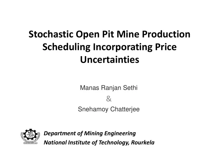
Stochastic Open Pit Mine Production Scheduling Incorporating Price h d li i i Uncertainties Uncertainties Manas Ranjan Sethi & Snehamoy Chatterjee Department of Mining Engineering Department of Mining Engineering National Institute of Technology, Rourkela

Introduction • Mine production scheduling is an assignment problem bl • Aim to maximizes profit • No algorithm is available to solve large scale mine scheduling problem scheduling problem • Number of approximate algorithms are available

Iron ore price 180 160 160 140 Price in US$ 120 per metric tonne 100 80 60 40 20 0 1980 1985 1990 1995 2000 2005 2010 2015 Year Year Fig: ‐ Iron ore price chart: 1982 ‐ 2011 Source: Index Mundi commodity price www.indexmundi.com/commodities/?commodity=iron ‐ ore&months=360

Stochastic production scheduling s T S N c     s i Maximize Z x   i t , t 1 (1 (1 r r ) )    t t 1 1 s 1 1 i i 1           s s s subject to x x 0, j , i N s , S t , T x {0,1}, i N s , S t , T i t , j t , i i t ,          s s x x x x 0, 0 i i N s N s , S t S t , T T  i t , 1 i t , N   st st st a x b S  i 1 i 1     s  x S i , N s , S t , T i 1 i t , s   s 1 1 N N   st st st a x b i 2 i 2  i 1  is the set of successor blocks of block i i i s c is the economic value of block for simulation i s i N is the number of blocks in the block model st a a is the amount of ore from a block of simulation at time is the amount of ore from a block x x of simulation s s at time t t i 1 i st a is the amount of waste from a block of simulation at time x s t i 2 i st b is the amount of ore production constraint from simulatio n at time s t 1 st st b 2 is the amount of waste production constraint from simulation at time s t T is the total number of production periods S is the number of simulation; is interest rate r

Constructing graph Three simulation with economic value of blocks 1 1 1 1 1 1 1 1 1 1 1 1 1 1 1 1 1 1 1 1 2 2 2 2 2 2 2 2 2 2 2 2 2 2 2 2 2 2 2 2 3 3 3 3 3 3 3 3 3 3 3 3 3 3 3 3 3 3 3 3 c 1 c 1 c 2 c 2 c 3 c 3 c 4 c 4 c 5 c 5 c 1 c 1 c 2 c 2 c 3 c 3 c 4 c 4 c 5 c 5 c 1 c 1 c 2 c 2 c 3 c 3 c 4 c 4 c 5 c 5 1 1 1 1 1 1 1 1 1 1 2 2 2 2 2 2 2 2 2 2 3 3 3 3 3 3 3 3 3 3 c 6 c 6 c 7 c 7 c 8 c 8 c 9 c 9 c 10 c 10 c 6 c 6 c 7 c 7 c 8 c 8 c 9 c 9 c 10 c 10 c 6 c 6 c 7 c 7 c 8 c 8 c 9 c 9 c 10 c 10 c 11 c 11 1 1 c 12 c 12 1 1 c 13 c 13 1 1 c 14 c 14 1 1 c 15 c 15 1 1 c 11 c 11 2 2 c 12 c 12 2 2 c 13 c 13 2 2 c 14 c 14 2 2 c 15 c 15 2 2 c 11 c 11 3 3 c 12 c 12 3 3 c 13 c 13 3 3 c 14 c 14 3 3 c 15 c 15 3 3 11 11 12 12 13 13 14 14 15 15 11 11 12 12 13 13 14 14 15 15 11 11 12 12 13 13 14 14 15 15 p y g  Economic value of blocks of three simulations after multiplying  1 1 1 1 1 1 1 1 1 1 2 2 2 2 2 2 2 2 2 2 d 1 d 1 d 2 d 2 d 3 d 3 d 4 d 4 d 5 d 5 d 1 d 1 d 2 d 2 d 3 d 3 d 4 d 4 d 5 d 5 3 3 3 3 3 3 3 3 3 3 d 1 d 1 d 2 d 2 d 3 d 3 d 4 d 4 d 5 d 5 d 6 d 6 1 1 d 7 d 7 1 1 d 8 d 8 1 1 d 9 d 9 1 1 d 10 d 10 1 1 d 6 d 6 2 2 d 7 d 7 2 2 d 8 d 8 2 2 d 9 d 9 2 2 d 10 d 10 2 2 d 6 d 6 d 6 d 6 3 3 d 7 d 7 d 7 d 7 3 3 d 8 d 8 d 8 d 8 3 3 d 9 d 9 d 9 d 9 3 3 d 10 d 10 d 10 d 10 3 3 6 6 7 7 8 8 9 9 10 10 6 6 7 7 8 8 9 9 10 10 d 11 d 11 1 1 d 12 d 12 1 1 d 13 d 13 1 1 d 14 d 14 1 1 d 15 d 15 1 1 d 11 d 11 2 2 d 12 d 12 2 2 d 13 d 13 2 2 d 14 d 14 2 2 d 15 d 15 2 2 d 11 d 11 3 3 d 12 d 12 3 3 d 13 d 13 3 3 d 14 d 14 3 3 d 15 d 15 3 3 Suppose economic value of blocks are Suppose economic value of blocks are 2 2 5 5 -2 -2 2 2 -2 -2 1 1 3 3 -1 -1 -2 -2 -2 -2 -6 -6 1 1 -3 -3 3 3 -2 -2 -3 -3 3 3 6 6 6 6 -1 -1 1 1 4 4 4 4 -2 -2 2 2 -1 -1 1 1 4 4 4 4 3 3 3 3 5 5 5 5 -1 -1 1 1 -2 -2 2 2 -1 -1 1 1 1 1 1 1 3 3 3 3 11 11 11 11 -5 -5 8 8 4 4 -7 -7 -4 -4 -3 -3 6 6 7 7 7 7 -3 -3 -1 -1 1 1 1 1 3 3 10 10

Constructing graph Merged graph Source 11 11 3 3 9 9 10 10 15 12 12 10 4 5 10 3 3 9 9 0 0 5 5 0 0 6 6 6 6 0 0 0 0 6 6 6 6 2 2 2 2 6 6 6 6 0 0 10 10 4 4 12 12 11 11 6 6 1 1 1 1 0 0 3 3 0 0 15 15 12 12 10 10 10 10 9 9 0 0 0 0 7 7 7 7 3 2 6 6 6 7 6 1 1 7 9 Sink

Case Study • A Iron ore deposit • Slope angle is 45 degree • 100 simulated ore body models • Price simulation was done using SGS algorithm

Variogram Model Nugget No of structure Sill Type Max Med Min 0 1 0.63 Spherical 100 70 27

3 ‐ D view of Pit

Conclusions • Production scheduling was performed by incorporating price uncertainty incorporating price uncertainty • The algorithm is computationally fast, so can handle large orebody model • No ultimate pit and pushback generation is o u t ate p t a d pus bac ge e at o s required in this algorithm • 5% more NPV can be generated as compared to conventional method conventional method

THANK YOU