Stereo Vision INEL 6088 - Computer Vision 1 Some References - PowerPoint PPT Presentation
Stereo Vision INEL 6088 - Computer Vision 1 Some References Secs.11.1 and 11.2 on Jain et. al. Davies, 4 th ed.: secs. 15.1-15.3 & 18.6-18.17 Davies, 3 rd ed.: secs.16.1-16.3 & 21.6-21.17 Chapter 11 on Szeliski's book
Stereo Vision INEL 6088 - Computer Vision � 1
Some References • Secs.11.1 and 11.2 on Jain et. al. • Davies, 4 th ed.: secs. 15.1-15.3 & 18.6-18.17 • Davies, 3 rd ed.: secs.16.1-16.3 & 21.6-21.17 • Chapter 11 on Szeliski's book 2
Stereo vision � 3
Epipolar plane and lines � Epipolar plane : plane passing through the camera centers and the feature point � Epipolar line : intersection between epipolar plane and image plane � Conjugate pair : two points in different images that are the projection of a single scene point � Disparity : difference in the conjugate pair’s pixel position if the images are superimposed � 4
Consideration of similar triangles gives � 5
Stereo Matching � Correspondence problem : main problem in stereo vision; to match a point in one image with the corresponding point in the other image. � Features that can be matched must be located. Sometimes they are created by lightening a pattern. � Depth is computed only for this features. Others are estimated by interpolation. � Epipolar constrain limits the search space � Obstruction means that points might be missing from one of the images – this makes solving the problem more difficult � 6
Baseline = 10in Taken with iPad (focal length = 3.2mm) P left = (1006, 641) P right = (691,635) � 7
x l - x r = 1006 - 691 pixels = 315 pixels Pixel size = 1.12 um x l - x r = 352.8 um = 0.3528 mm Baseline = 10in Z = (10in)(3.3mm)/(.3528mm) = 93.5 in Actual distance = 70 in (measured with tape) Difference is to large. Error due to small device rotation? � 8
lc2=im2(411:962,449:1000); crop_im1 = im1(529:579,976:1026); � 9
xc12 = normxcorr2(double(crop_im1),double(lc2)); plot(max(xc12)); figure; plot(max(xc12')); figure; imshow(lc2) figure; imshow(crop_im1) peaks at (257,159) � 10
� 11
Common metrics to compare image patches: • Sum of square di ff erences: � � ( I l − I r ) 2 • Absolute di ff erence: � � | I l − I r | • Cross-correlation: � � I l I r � � I l I r • Normalized Cross-correlation √ � I 2 � I 2 r l See this link for other similarity measures. � 12
� 13
Solutions to the Correspondence problem � Edge Matching � Filter each image with a Gaussian at four different scales � Compute edge positions within row � Match non-horizontal edges by comparing orientation and magnitude � Refine disparity estimates by using finer scales � However, strong edges tend to be silhouette edges and correspond to different parts of the object in the two images � 14
Region Correlation � Match areas of the image with high variance � Calculate variance along different directions using all pixels in a window centered about a point. � Select minimum value as the interest value of the central pixel � Chose pixels whose interest measure is a local maxima and is above a threshold as the feature points � Compute correlation coefficient between a small window of pixels centered around the selected features � Consider only features that satisfy the epipolar constrain � Features with highest correlation coefficient are considered a match � 15
Directional variances: look for points with large min(I 1 , I 2 , I 3 , I 4 ) Correlation coefficient: match if r>th - look along epipolar lines � 16
Other feature based methods � edge points � lines (length, orientation, midpoint, average contrast) � corners � points where edge lines meet � formed by intensity patterns � select method based on � kind of object of interest and � illumination � image contrast, etc. � 17
Epipolar lines generalized � 18
p l = f l P l Z l p r = f r P r Z r 19
Rectification • Transformation to make epipolar lines collinear and parallel to horizontal axis • Steps: • Rotate left camera so that epipole goes to infinity along the horizontal axis • Apply the same rotation to right camera • Rotate right camera by R • Adjust scale in both camera reference frames 20
Rectification • Rectification: make the epipolar lines collinear and parallel to the hori- zontal image axis • This transformation can be described in terms of the matrix R defined in the equation P r = R ( P l − T ) and a rotation matrix Q such that the epipolar lines become parallel. • Assume same f for both cameras. • The Q is a 3 × 3 matrix given by ⇤ T ⇥ q T q T q T Q = 1 2 3 where T q 1 = � � � T � ⇤ T ⇥ 0 − T 2 , T 1 , q 2 = p T 2 1 + T 2 2 and q 3 = q 1 × q 2 21
Rectification 1. For each left-camera point p l = [ x, y, f ] T compute [ x � , y � , z � ] = Qp l and the coordinates of the corresponding rectified point p � l , l = f p � z � [ x � , y � , z � ] 2. Let R r = RQ . 3. Repeat step 1 for the right-camera using R r and p r . 22
23
Essential and Fundamental Matrices • A translation vector T = O r − O l and an orthogonal rotational matrix R bring the left camera’s coordinate system into the right’s. P r = R ( P l − T ) • Since P l and T are in Π e , P l − T is also in Π e • Thus ( P l − T ) · ( T × P l ) = 0 • From the definition of the cross product, a matrix A can be defined � � T 1 T 2 T 3 � � � � = T × P l P l 1 P l 2 P l 3 � � � � i j k � � = i ( T 2 P l 3 − T 3 P l 2 ) − j ( T 1 P l 3 − T 3 P l 1 ) + k ( T 1 P l 2 − T 2 P l 1 ) 2 3 2 3 2 3 2 3 − T 3 P l 2 + T 2 P l 3 0 i − T 3 T 2 P l 1 i 5 = 5 = AP l = 0 T 3 P l 1 − T 1 P l 3 j T 3 − T 1 P l 2 j 4 5 4 4 5 4 − T 2 P l 1 + T 1 P l 2 0 k − T 2 T 1 P l 3 k 24
• The previous result in step 2 can be expressed as ( R − 1 P r ) T AP l = 0 • Since R is orthogonal, R T = R − 1 . • In general, ( AB ) T = B T A T • Thus P T r RAP l = P T r EP l = 0 • The essential matrix is E = RA • The image points p l and p r are also related by E p T r Ep l = 0 25
• The pixel coordinates of a given point p k are given by c p k = M int,k p k where M int,k is a matrix that represent the intrinsic parameters. • The above expression p T r Ep l = 0 p r ) T EM − 1 ( M − 1 int,r c int,l b p l = 0 T M − T int,r EM − 1 c int,l b p l = 0 p r T F b c p l = 0 p r • The fundamental matrix F = M − T int,r EM − 1 int,l describes the epipolar geom- etry in terms of pixel coordinates. • The essential matrix is defined in terms of camera coordinates. • The essential matrix depends on the extrinsic parameters. 26
F � p l describes the epipolar line on which the corresponding point � p r on the other image must lie. MATLAB page on how to obtain the epipolar line from the Fundamental matrix 27
Reconstruction • by triangulation - possible if intrinsic and extrinsic parameters are known • up to a scale factor - intrinsic parameters are known 28
29
Reconstruction by Triangulation • Assume that: stereo system’s intrinsic and extrinsic parameters are known. • Compute: 3-D location for points from their projections p l and p r • A point P lies in the intersection of the rays from O l and p l , and O r and p r • Problem: since parameters and image locations are known only approxi- mately, the two rays will not intersect • Solution: estimate the intersection as the point of minimum distance from both rays. • Let – a p l be the ray l going from O l through p l – T + bR T p r be the ray, r, through O r through p r expressed in the left reference frame. – w be a vector orthogonal to both l and r • Problem reduces to finding the midpoint , P 0 , of the segment parallel to w that joins l and r 30
• w can be expressed as w = p l × R T p r • a p l + c w represent a line through a p l parallel to w . • Determine the endpoints of the segment, s , belonging to the line parallel to w that joins l ( a 0 p l ) and r ( T + b 0 R T p r ) from a p l − ( T + bR T p r ) + c w = 0 by solving a p l − bR T p r + c ( p l × R T p r ) = T for a 0 , b 0 and c 0 • The triangulated point P 0 is the midpoint of s . 31
Zero disparity means that the point is on the surface; positive disparity indicates points farther than the surface, etc. ACTIVE VISION SYSTEM- camera is controlled dynamically by the analysis algorithm to facilitate depth (or other) computation. � 32
Recommend
More recommend
Explore More Topics
Stay informed with curated content and fresh updates.
