Depth from Stereo Dominic Cheng February 7, 2018 Agenda 1. - PowerPoint PPT Presentation
Depth from Stereo Dominic Cheng February 7, 2018 Agenda 1. Introduction to stereo 2. Efficient Deep Learning for Stereo Matching (W. Luo, A. Schwing, and R. Urtasun. In CVPR 2016.) 3. Cascade Residual Learning: A Two-stage Convolutional
Depth from Stereo Dominic Cheng February 7, 2018
Agenda 1. Introduction to stereo 2. Efficient Deep Learning for Stereo Matching (W. Luo, A. Schwing, and R. Urtasun. In CVPR 2016.) 3. Cascade Residual Learning: A Two-stage Convolutional Neural Network for Stereo Matching (J. Pang, W. Sun, J. SJ. Ren, C. Yang, and Q. Yan. In CVPR 2017.)
Introduction to Stereo
What is stereo? Depth from images is a very intuitive ability Given two images of a scene from (slightly) different ● viewpoints, we are able to infer depth Can we do the same using computers? Yes (kind of?) ● First, we need to appreciate the geometry of the situation ● Source: https://s.hswstatic.com/gif/pc-3-d-brain.jpg
Geometry in stereo (a visual overview) Think of images as projections of 3D points ● (in the real world) onto a 2D surface (image plane) X L is the projection of X, X 1 , X 2 , X 3 , .... onto the ● left image X, X 1 , X 2 , X 3 will also project onto the right ● image Source: https://upload.wikimedia.org/wikipedia/commons/thumb/1/14/Epipolar_geometry.svg/6 40px-Epipolar_geometry.svg.png?1517775941158
Geometry in stereo (a visual overview) What do you notice? ● Projections of X 1 , X 2 , X 3 on right image all lie ● on a line This line is known as an epipolar line ● Points e L , e R are known as epipoles ○ Projections of cameras’ optical centers O L , O R ○ onto the images All epipolar lines will intersect at epipoles ○ Left image has corresponding epipolar line ○ Geometry of stereo vision also known as ● epipolar geometry Source: https://upload.wikimedia.org/wikipedia/commons/thumb/1/14/Epipolar_geometry.svg/6 40px-Epipolar_geometry.svg.png?1517775941158
Geometry in stereo (a visual overview) What does this give us? ● All 3D points that could have resulted in X L ● must have a projection on the right image, and must be on the epipolar line e R − x R Given just the left/right images and X L , you ● can search on the corresponding epipolar line in the right image. If you can find the corresponding match X R , you can uniquely determine the 3D position of X. Source: https://upload.wikimedia.org/wikipedia/commons/thumb/1/14/Epipolar_geometry.svg/6 40px-Epipolar_geometry.svg.png?1517775941158
Geometry in stereo (a visual overview) In practice ... ● Epipolar lines can be ● made parallel through a process called rectification Simplifies the process ● of finding a match and calculating the 3D point Credit: S. Savarese Source: http://web.stanford.edu/class/cs231a/lectures/lecture6_stereo_systems.pdf
Geometry in stereo (a visual overview) How do you actually get depth? ● If you find correspondences x and x’, the ● quantity x− x’ is known as the disparity By similar triangles, you can convince yourself ● that disparity is inversely proportional to depth Problem statement, reformulated: Find the ● disparity for every pixel in the left (or right) image by finding matches in the right (or left) image Credit: L. Shapiro Source: https://courses.cs.washington.edu/courses/cse455/16wi/notes/11_Stereo.pdf
Practical example: KITTI Source: KITTI Stereo 2015 Training Set [5]
Efficient Deep Learning for Stereo Matching [1] W. Luo, A. Schwing, and R. Urtasun. In CVPR 2016.
Features for stereo correspondence Finding a good match is hard ● What is a good feature? ● Can we learn the features ● instead? Source: https://upload.wikimedia.org/wikipedia/en/3/3b/Stereo_empire.jpg
Key idea Construct a neural network that takes input ● images (left/right) and produces representative features that can be used to find stereo correspondences efficiently.
Network architecture Siamese network ● Shared weights enforce similar features are ○ learned on both left/right images Several convolution layers ● Paper implements a fairly vanilla network ○ Several variants are tested; the key behind the ○ choices of kernel size / stride is the effective receptive field
Training Pose this as a multi-class classification problem ● Differentiating from earlier work which poses as ○ binary classification [3] Left image patch is equal to the receptive field ● Final feature volume after passing through the ○ network is 1 x 1 x 64 (H x W x C) Right patch is larger to accommodate more ● context across range of possible disparities Final feature volume is 1 x S x 64 (S is total number ○ of search locations) Inner product of left feature with every spatial ● location of right feature ⇒ S scores
Training Multi-class cross entropy loss over these S scores ● Each class is an actual spatial bin ● Probability mass is diffused across ground truth ● bin +/- 2 bins, to allow for some ambiguity
Testing Does not have to take the same form as training ● Efficiency comes from enforcing that similarity ● between features is measured by their inner product Can compute all these features at once on ● left/right images Produce a cost volume by computing similarity ● across multiple disparities H x W x D, where D is number of disparity ○ candidates
Smoothing How to get final result? ● Could just take most likely assignments across this volume ● Drawback: These predictions tend to be rough (no smoothness prior) ● Can smooth in various ways through averaging, energy minimization (semi-global block matching), ● slanted-plane, and other post-processing techniques
Evaluation Train and test on KITTI only (training set has 200 image pairs) ● Very straightforward training procedure ● Competitive results (on D1 error reported by testbench) with significant speed-up ● Highlighting similar approach of [3] ○
Source:http://www.cvlibs.net/datasets/kitti/eval_scene_flow_detail.php?benchmark=ste reo&result=b54624a9eed52b4c8e6c76b411179dce4bd7d4d8 Sample output ● From submission to KITTI 2015 stereo benchmark ● Middle is prediction, bottom is error ● Even small differences in prediction can result in large disparity errors
Cascade Residual Learning: A Two- stage Convolutional Neural Network for Stereo Matching [2] J. Pang, W. Sun, J. SJ. Ren, C. Yang, and Q. Yan. In CVPR 2017.
Another approach This can be posed as a classification problem, why not regression? ● Based on idea of DispNet presented in [4] ○ Feed two images in, get dense disparity prediction out ○ Advantage: ● Note that in previous approach, smoothing was still necessary for good results ○ We could try to make the entire prediction process end-to-end learnable ○ Disadvantage: ● Do not get to explicitly incorporate geometric priors ○
Architecture Two parts ● DispFulNet: Predict initial disparity ○ DispResNet: Refine the prediction ○
Architecture DispFulNet ● Based on DispNet [4] ○ Encoder/decoder architecture; take left/right images as input, share lower level features, combine, predict ○ Train with L 1 loss against ground truth disparity map ○ Make predictions at multiple scales during decode (d 1 (S) , …, d 1 (0) ) ○ ○ Produce initial disparity map d 1
Architecture DispResNet ● Idea from ResNet ○ Given initial prediction, have another network predict the residuals ○ Again, produce predictions at multiple scales to incorporate more supervision ○ Output is final disparity ○
Evaluation Train on a lot of data ● FlyingThings3D: Synthetic dataset with ○ 22k+/4k+ train/test examples Finetuning on KITTI ○ Test on FlyingThings, Middlebury, and KITTI ● Currently #8 on KITTI 2015 stereo ● leaderboard! Keep in mind submitted March 2017 ○
Evaluation Qualitative assessment of refinement ●
Source:http://www.cvlibs.net/datasets/kitti/eval_scene_flow_detail.php?benchmark=ste reo&result=f791987e39ecb04c1eee821ae3a0cd53d5fd28c4 Sample output ● From submission to KITTI 2015 stereo benchmark ● Middle is prediction, bottom is error ● Generally smoother outputs with ability to define sharp boundaries for objects
Questions
References [1] W. Luo, A. Schwing, and R. Urtasun, “Efficient deep learning for stereo matching,” in International Conference on Computer Vi sion and Pattern Recognition (CVPR), 2016. [2] J. Pang, W. Sun, J. S. Ren, C. Yang, and Q. Yan, “Cascade residual learning: A two -stage convolutional neural network for stereo matching,” in ICCV Workshop on Geometry Meets Deep Learning, Oct 2017. [3] J. Zbontar and Y. LeCun, “Stereo matching by training a convolutional neural network to compare image patches,” Journal of Ma chine Learning Research, vol. 17, pp. 1 – 32, 2016. [4] N.Mayer, E.Ilg, P.Häusser, P.Fischer, D.Cremers, A.Dosovitskiy, and T.Brox, “A large dataset to train convolutional networks for disparity, optical flow, and scene flow estimation,” in IEEE International Conference on Computer Vision and Pattern Recognition (CVPR), 2016. arXiv:1512.02134. [5] M. Menze and A. Geiger, “Object scene flow for autonomous vehicles,” in Conference on Computer Vision and Pattern Recognition (CVPR), 2015.
Recommend
More recommend
Explore More Topics
Stay informed with curated content and fresh updates.
