Stereo Computer Vision Fall 2018 Columbia University Homework - PowerPoint PPT Presentation
Stereo Computer Vision Fall 2018 Columbia University Homework Homework 2 grades are back Median 37/40, std 7.2 Homework 3 due now Homework 4 out today My Office Hours Now Mondays 5pm-6pm Course Evaluations 60% response
Stereo Computer Vision Fall 2018 Columbia University
Homework • Homework 2 grades are back • Median 37/40, std 7.2 • Homework 3 due now • Homework 4 out today
My Office Hours • Now Mondays 5pm-6pm
Course Evaluations • 60% response rate so far • Please respond by tomorrow • We read all feedback!
Image Stitching
Image alignment Why don’t these image line up exactly?
Transformation Models • T ranslation only • Rigid body (translate+rotate) • Similarity (translate+rotate+scale) • AIne • Homography (projective)
Camera Projection X r 11 r 12 r 13 t x f 0 0 x ˜ Y r 21 r 22 r 23 t y y ˜ = f 0 0 Z r 31 r 32 r 33 t x z ˜ 0 0 1 1 Camera Camera World Intrinsics Extrinsics Coordinates
Camera Matrix Mapping points from the world to image coordinates is matrix multiplication in homogenous coordinates X C 11 C 12 C 13 C 14 x ˜ Y y ˜ C 21 C 22 C 23 C 24 = Z z ˜ C 31 C 32 C 33 C 34 1
Projection of 3D Plane All points on the plane have Z = 0 X C 11 C 12 C 13 C 14 x ˜ Y y ˜ C 21 C 22 C 23 C 24 = 0 z ˜ C 31 C 32 C 33 1 1 Slide credit: Peter Corke
Projection of 3D Plane All points on the plane have Z = 0 X C 11 C 12 0 C 14 x ˜ Y y ˜ C 21 C 22 0 C 24 = 0 z ˜ C 31 C 32 0 1 1 Slide credit: Peter Corke
Two-views of Plane = H 1 ( = H 2 ( x 1 ˜ x 2 ˜ 1 ) 1 ) X X y 1 ˜ y 2 ˜ Y Y z 1 ˜ z 2 ˜ x 2 ˜ x 1 ˜ = H 2 H − 1 y 2 ˜ y 1 ˜ 1 z 2 ˜ z 1 ˜ Slide credit: Deva Ramanan
Image Alignment Algorithm Given images A and B 1. Compute image features for A and B 2. Match features between A and B 3. Compute homography between A and B using least squares on set of matches What could go wrong? Slide credit: Noah Snavely
Outliers outliers inliers Slide credit: Noah Snavely
Robustness • Let’s consider a simpler example… linear regression Problem: Fit a line to these datapoints Least squares fit • How can we fix this? Slide credit: Noah Snavely
We need a better cost function… • Suggestions? Slide credit: Noah Snavely
Counting inliers Slide credit: Noah Snavely
Counting inliers Inliers: 3 Slide credit: Noah Snavely
Counting inliers Inliers: 20 Slide credit: Noah Snavely
Idea • Given a hypothesized line • Count the number of points that “agree” with the line – “Agree” = within a small distance of the line – I.e., the inliers to that line • For all possible lines, select the one with the largest number of inliers Slide credit: Noah Snavely
How do we find the best line? • Unlike least-squares, no simple closed-form solution • Hypothesize-and-test – Try out many lines, keep the best one – Which lines? Slide credit: Noah Snavely
RANSAC (RANdom SAmple Consensus) : Fischler & Bolles in ‘81. Algorithm: 1. Sample (randomly) the number of points s required to fit the model 2. Solve for model parameters using samples 3. Score by the fraction of inliers within a preset threshold of the model Repeat 1-3 until the best model is found with high confidence Slide credit: James Hays
RANSAC Line fitting example Algorithm: 1. Sample (randomly) the number of points required to fit the model (s=2) 2. Solve for model parameters using samples 3. Score by the fraction of inliers within a preset threshold of the model Repeat 1-3 until the best model is found with high confidence Illustration by Savarese
RANSAC Line fitting example Algorithm: 1. Sample (randomly) the number of points required to fit the model ( s =2) 2. Solve for model parameters using samples 3. Score by the fraction of inliers within a preset threshold of the model Repeat 1-3 until the best model is found with high confidence Slide credit: James Hays
RANSAC Line fitting example � N 6 Inliers � Algorithm: 1. Sample (randomly) the number of points required to fit the model ( s =2) 2. Solve for model parameters using samples 3. Score by the fraction of inliers within a preset threshold of the model Repeat 1-3 until the best model is found with high confidence Slide credit: James Hays
RANSAC � � N 14 Inliers Algorithm: 1. Sample (randomly) the number of points required to fit the model ( s =2) 2. Solve for model parameters using samples 3. Score by the fraction of inliers within a preset threshold of the model Repeat 1-3 until the best model is found with high confidence Slide credit: James Hays
RANSAC for alignment Slide credit: Deva Ramanan
RANSAC for alignment Slide credit: Deva Ramanan
RANSAC for alignment Slide credit: Deva Ramanan
Implementing image warping • Given a coordinate xform ( x’ , y ’ ) = T ( x,y ) and a source image f ( x,y ), how do we compute an xformed image g ( x’ , y ’ ) = f ( T ( x , y ))? T ( x,y ) y’ y x x’ f ( x,y ) g ( x’,y’ )
Forward Warping • Send each pixel f ( x ) to its corresponding location ( x’ , y ’ ) = T ( x , y ) in g ( x’ , y ’ ) • What if pixel lands “between” two pixels? T ( x,y ) y’ y x x’ f ( x,y ) g ( x’,y’ )
Inverse Warping • Get each pixel g ( x’,y’ ) from its corresponding location ( x,y ) = T -1 ( x,y ) in f ( x,y ) • Requires taking the inverse of the transform • What if pixel comes from “between” two pixels? T -1 ( x,y ) y’ y x x’ f ( x,y ) g ( x’,y’ )
Inverse Warping • Get each pixel g ( x’ ) from its corresponding location x’ = h ( x ) in f ( x ) • What if pixel comes from “between” two pixels? • Answer: resample color value from interpolated ( prefiltered ) source image T -1 ( x,y ) y’ y x x’ f ( x,y ) g ( x’,y’ )
Blending • We’ve aligned the images – now what? Slide credit: Noah Snavely
Blending • Want to seamlessly blend them together Slide credit: Noah Snavely
Image Blending Slide credit: Noah Snavely
Feathering + 1 1 0 0 = Slide credit: Noah Snavely
Effect of window size 1 1 left right 0 0 Slide credit: Noah Snavely
Effect of window size 1 1 0 0 Slide credit: Noah Snavely
Blending Slide credit: Davis ‘98
Blending Slide credit: Olga Russakovsky
Blending Slide credit: Davis ‘98
Stereo
Stereo vision ~50cm ~6cm � 44 Slide credit: Antonio Torralba
Why not put our second eye here?
Stereoscopes: A 19 th Century Pastime
Public Library, Stereoscopic Looking Room, Chicago, by Phillips, 1923
Teesta suspension bridge-Darjeeling, India
Mark Twain at Pool Table", no date, UCR Museum of Photography
3D Movies
Depth without objects Random dot stereograms (Bela Julesz) Julesz, 1971 � 51
Stereo • Given two images from different viewpoints – How can we compute the depth of each point in the image? – Based on how much each pixel moves between the two images
Geometry for a simple stereo system Z 1 x L f X 1 � 53 Slide credit: Antonio Torralba
Geometry for a simple stereo system Z 1 Z? x L f X 1 � 54 Slide credit: Antonio Torralba
Geometry for a simple stereo system Z 1 Z 2 Z? x L x R f f X 1 X 2 T � 55 Slide credit: Antonio Torralba
Geometry for a simple stereo system Z 1 Z 2 Z? x L x R f f X 1 X 2 T � 56 Similar triangles Slide credit: Antonio Torralba
Geometry for a simple stereo system Z 1 Z 2 Z? x L x R f f X 1 X 2 T � 57 Similar triangles Slide credit: Antonio Torralba
Geometry for a simple stereo system Z 1 Z 2 Similar triangles: Z? T+X L -X R = x R x L Z-f f f X 1 X 2 T Slide credit: Antonio Torralba
Geometry for a simple stereo system Z 1 Z 2 Similar triangles: Z? T+X L -X R T = x R x L Z-f Z f f X 1 X 2 T � 59 Slide credit: Antonio Torralba
Geometry for a simple stereo system Z 1 Z 2 Similar triangles: Z? T+X L -X R T = x R x L Z-f Z f f X 1 X 2 Solving for Z: T T Z = f X R - X L Disparity � 60 Slide credit: Antonio Torralba
Epipolar geometry epipolar lines (x 2 , y 1 ) (x 1 , y 1 ) Two images captured by a purely horizontal translating camera ( rectified stereo pair) x 2 -x 1 = the disparity of pixel (x 1 , y 1 ) Slide credit: Noah Snavely
Your basic stereo algorithm For each epipolar line For each pixel in the left image • compare with every pixel on same epipolar line in right image • pick pixel with minimum match cost Improvement: match windows Slide credit: Noah Snavely
Stereo matching based on SSD SSD d min d Best matching disparity Slide credit: Noah Snavely
Window size W = 3 W = 20 Effect of window size Better results with adaptive window – Smaller window • T. Kanade and M. Okutomi, A Stereo Matching Algorithm + with an Adaptive Window: Theory and Experiment ,, Proc. International Conference on Robotics and • Automation, 1991. – Larger window • D. Scharstein and R. Szeliski. Stereo matching with nonlinear diffusion. International Journal of Computer + Vision, 28(2):155-174, July 1998 • Slide credit: Noah Snavely
Stereo results – Data from University of Tsukuba – Similar results on other images without ground truth Scene Ground truth Slide credit: Noah Snavely
Recommend
More recommend
Explore More Topics
Stay informed with curated content and fresh updates.
