Steiner Forest (Approximation Algorithms by V. Vazirani, Chapter 22) - PowerPoint PPT Presentation

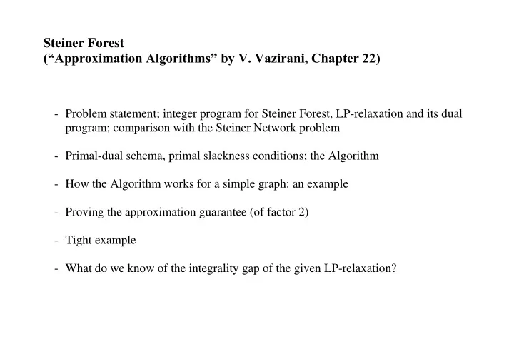
Steiner Forest (“Approximation Algorithms” by V. Vazirani, Chapter 22) - Problem statement; integer program for Steiner Forest, LP-relaxation and its dual program; comparison with the Steiner Network problem - Primal-dual schema, primal slackness conditions; the Algorithm - How the Algorithm works for a simple graph: an example - Proving the approximation guarantee (of factor 2) - Tight example - What do we know of the integrality gap of the given LP-relaxation?

Steiner Forest problem Let G = ( V , E ) be an undirected graph with a cost function on the edges c : E  Q + . Given a collection of disjoint subsets of V : S 1 , …, S k , we are to find a minimum cost subgraph in which any pair of vertices from the same set S i is connected. [In general, such a subgraph may not exist at all if G is not connected.] Obviously, the solution is a forest. We will start with defining a connectivity requirement function r : V x V  {0, 1} 1, if u and v belong to the same set S i r ( u , v ) = 0, otherwise To restate the problem as an integer program, we will consider cuts ( S , S c ) in G and think of edges that should be chosen in their boundaries  ( S , S c ) to satisfy the connectivity requirements. [We may also use just S to refer to the cut ( S , S c ).]

Let’ s define a function on all cuts in G that “selects” the cuts in the boundaries of which we must choose at least one edge. 1, if there exist u in S and v in S c such that r ( u , v ) = 1 f ( S , S c ) = 0, otherwise Now, here’s the integer program for Steiner Forest: minimize  e  E c e x e subject to  e  ( S ) x e  f ( S , S c ), for each cut ( S , S c ) x e  {0, 1}, e  E To get the LP-relaxation, we simply change the last set of conditions to x e  0, e  E Note that the conditions x e  1 are clearly redundant.

The number of constraints in our integer and linear programs is exponential. However, we’re not going to solve the linear program, we will use the primal -dual schema instead, so the exponential number of constraints is not a concern. This is in contrast with the approach to the Steiner Network problem that will be discussed in the next talk. Since we will use iterated LP-rounding there, we will have to deal with the large number of constraints issue. Let us now state the dual program: maximize  S   V f ( S )  y S subject to  S:e  ( S ) y S  c e , for each e  E y S  0, S  V

Applying the primal-dual schema Primal-dual schema: an integral solution to the primal program and a feasible solution to the dual program are constructed iteratively. Our algorithm will be guided by (a) the slackness conditions, with the dual solution optimality being the goal, and (b) by the primal program constraints, with the primal solution feasibility being the goal, in turn. So, we start with null primal and dual solutions and will, in turn, “raise” variables y S corresponding to appropriate cuts, and pick appropriate edges, setting their variables x e to 1. [Note that, surely, there is no point in raising variables of cuts with f ( S , S c ) = 0.] Here are the slackness conditions for the dual solution:  S:e  ( S ) y S = c e , for each e  E with x e = 1. (Every picked edge is “tight”.) The other set of the slackness conditions would require us to pick exactly one edge in the boundary of each cut ( S , S c ) with y S > 0. That we cannot achieve, but we will be able to upper bound the number of edges selected in the boundaries on average .

Now, the main questions are: - which cuts to raise in a given iteration? - which edge to pick in a given iteration? When we raise certain cuts, we must stop at the point when at least one edge in their boundaries becomes “tight”, that is, the slackness condition for that edge is satisfied. Naturally, we would then pick the newly-tight edge. Clearly, it makes sense to raise only “unsatisfied” cuts, since we do not want to pick edges in the boundaries of the already satisfied ones. But not all of them, as that would make it very hard to track the process. A natural choice then is to raise, in a given iteration, only such unsatisfied cuts ( S , S c ) that either S or S c is a minimal (w.r.t. inclusion) unsatisfied set. We will call such cuts (and respective minimal sets) “active”. It is easy to keep track of the currently active cuts and detect edges in their boundaries that get tight when variables y S for the active cuts are raised in a synchronized manner.

The following characterization of active sets is a key ingredient in the algorithm design: Set S is active iff ( S , S c ) is unsatisfied and S is a connected component in the currently picked subgraph. Since we always pick edges in the boundaries of the currently active sets, our picked subgraph is always a forest. Now, here is the algorithm: 1. Initialize all the primal and dual programs’ variables to zeros. 2. While (there exists an unsatisfied set) do simultaneously raise y S for each active set S until some edge e goes tight Select e by setting x e to 1. 3. Remove all the unnecessary selected edges. - Some implementation details (tracking active sets, etc.). - Why we end up with feasible primal and dual solutions. - Why we can simultaneously remove all the unnecessary edges in step (3).

Example u 20 v 6 6 a 9 b 16 19 12 12 s t The connectivity requirements: r ( u , v ) = 1, r ( s , t ) = 1

The approximation guarantee We denote by F the forest obtained at the end of step 2, and by F’ – the final solution after step 3. Let deg F’ ( S ) denote the number of edges of F’ crossing the cut ( S , S c ). Lemma Let C be any subset of V . If f ( C ) = 0, then deg F’ ( C )  1. In particular, this is true for the set of vertices of any connected component at any iteration of the algorithm (w.r.t. the currently picked edges). Theorem The algorithm achieves an approximation guarantee of factor 2. Proof Since the objective function of any feasible solution to the dual problem gives a lower bound for the primal problem optimum, it suffices to show  e  E’ c e  2  S  V y S ( = 2  S  V f ( S )  y S ) For the left-hand side, we notice that every picked edge is tight. Then, what we need is:  S  V deg F’ ( S )  y S  2  S  V y S .

We will show more: in each iteration of the algorithm, the left-hand side of the last inequality grows no more than its right-hand side. That is equivalent to proving the following bound:  S active deg F’ ( S )  2 (# of active sets) So, we want to upper b ound the average degree of the active sets…

Tight example is the one for the metric Steiner tree problem: K n +1 , S 1 contains n vertices, edges in S 1 of cost 2, the remaining edges of cost (1 +  ). Integrality gap Claim The algorithm places an upper bound of 2 on the integrality gap of the LP-relaxation of the Steiner forest problem. That is, sup I OPT( I ) / LP-OPT( I )  2. Why? Here is an example that places a lower bound of (essentially) 2 on the integrality gap in question: Given a cycle on n vertices, with all the edges of cost 1, we are to find the minimum spanning tree. The MST cost is obviously ( n – 1). Our algorithm will find a dual of value n /2. There is also a fractional primal solution of the same value: take all the edges with the coefficient of 1/2. So, that must be LP-OPT for the given instance.