Statistical methods for neural decoding Liam Paninski Gatsby - PowerPoint PPT Presentation
Statistical methods for neural decoding Liam Paninski Gatsby Computational Neuroscience Unit University College London http://www.gatsby.ucl.ac.uk/ liam liam@gatsby.ucl.ac.uk November 9, 2004 Review... x ? y
Statistical methods for neural decoding Liam Paninski Gatsby Computational Neuroscience Unit University College London http://www.gatsby.ucl.ac.uk/ ∼ liam liam@gatsby.ucl.ac.uk November 9, 2004
Review... x ? y ������� ��������������� ...discussed encoding: p ( spikes | � x )
Decoding Turn problem around: given spikes, estimate input � x . What information can be extracted from spike trains — by “downstream” areas? — by experimenter? Optimal design of neural prosthetic devices.
Decoding examples Hippocampal place cells: how is location coded in populations of cells? Retinal ganglion cells: what information is extracted from a visual scene and sent on to the brain? What information is discarded? Motor cortex: how can we extract as much information from a collection of MI cells as possible?
Discrimination vs. decoding Discrimination: distinguish between one of two alternatives — e.g., detection of “stimulus” or “no stimulus” General case: estimation of continuous quantities — e.g., stimulus intensity Same basic problem, but slightly different methods...
Decoding methods: discrimination Classic problem: stimulus detection. Data: 2 trial 1 0 0.1 0.2 0.3 0.4 0.5 0.6 0.7 0.8 0.9 1 time (sec) Was stimulus on or off in trial 1? In trial 2?
Decoding methods: discrimination Helps to have encoding model p ( N spikes | stim ): stim off stim on 0.25 0.2 0.15 p(N) 0.1 0.05 0 5 10 15 N
Discriminability discriminability depends on two factors: — noise in two conditions — separation of means “ d ′ ” = separation / spread = signal / noise
Poisson example Discriminability d ′ = | µ 0 − µ 1 | ∼ | λ 0 − λ 1 | √ σ λ Much easier to distinguish Poiss (1) from Poiss (2) than Poiss (99) from Poiss (100). — d ′ ∼ 1 = 1 vs. d ′ ∼ 1 1 100 = . 1 √ √ √ Signal to noise increases like | Tλ 0 − Tλ 1 | ∼ T : speed-accuracy √ Tλ tradeoff
Discrimination errors
Optimal discrimination What is optimal? Maximize hit rate or minimize false alarm?
Optimal discrimination: decision theory Write down explicit loss function, choose behavior to minimize expected loss Two-choice loss L ( θ, ˆ θ ) specified by four numbers: — L (0 , 0): correct, θ = ˆ θ = 0 — L (1 , 1): correct, θ = ˆ θ = 1 — L (1 , 0): missed stimulus — L (0 , 1): false alarm
Optimal discrimination Denote q ( data ) = p (ˆ θ = 1 | data ). Choose q ( data ) to minimize E p ( θ | data ) ( L ( θ, ˆ θ )) ∼ � � � p ( θ ) p ( data | θ ) q ( data ) L ( θ, 1) + (1 − q ( data )) L ( θ, 0) θ (Exercise: compute optimal q ( data ); prove that optimum exists and is unique.)
Optimal discrimination: likelihood ratios It turns out that optimal � p ( data | θ = 1) � q opt ( data ) = 1 : p ( data | θ = 0) > T likelihood-based thresholding. Threshold T depends on prior p ( θ ) and loss L ( θ, ˆ θ ). — Deterministic solution: always pick the stimulus with higher weighted likelihood, no matter how close — All information in data is encapsulated in likelihood ratio. — Note relevance of encoding model p ( spikes | stim ) = p ( data | θ )
Likelihood ratio stim off 0.25 stim on 0.2 p(N) 0.15 0.1 0.05 0 5 10 15 20 p(N | off) / p(N | on) 15 10 5 0 5 10 15 N
Poisson case: full likelihood ratio Given spikes at { t i } , λ stim ( t ) dt � R likelihood = e − λ stim ( t i ) i Log-likelihood ratio: � log λ 0 � ( λ 1 ( t ) − λ 0 ( t )) dt + ( t i ) λ 1 i
Poisson case � log λ 0 � ( λ 1 ( t ) − λ 0 ( t )) dt + ( t i ) λ 1 i Plug in homogeneous case: λ j ( t ) = λ j . K + N log λ 0 λ 1 Counting spikes not a bad idea if spikes are really a homogeneous Poisson process; here N = a “sufficient statistic.” — But in general, good to keep track of when spikes arrive. (The generalization to multiple cells should be clear.)
Discriminability: multiple dimensions Examples: synaptic failure, photon capture (Field and Rieke, 2002), spike clustering 1-D: threshold separates two means. > 1 D?
Multidimensional Gaussian example Look at log-likelihood ratio: Z exp[ − 1 1 µ 1 ) t C − 1 ( � 2 ( � x − � x − � µ 1 )] log Z exp[ − 1 1 µ 0 ) t C − 1 ( � 2 ( � x − � x − � µ 0 )] = 1 µ 0 ) t C − 1 ( � µ 1 ) t C − 1 ( � 2[( � x − � x − � µ 0 ) − ( � x − � x − � µ 1 )] = C − 1 ( � µ 1 − � µ 0 ) · � x Likelihood ratio depends on � x only through projection C − 1 ( � µ 1 − � µ 0 ) · � x ; thus, threshold just looks at this projection, too — same regression-like formula we’re used to. C white: projection onto differences of means What happens when covariance in two conditions is different? (exercise)
Likelihood-based discrimination Using correct model is essential (Pillow et al., 2004): — ML methods are only optimal if model describes data well
Nonparametric discrimination (Eichhorn et al., 2004) examines various classification algorithms from machine learning (SVM, nearest neighbor, Gaussian processes). Reports significant improvement over “optimal” Bayesian approach under simple encoding models — errors in estimating encoding model? — errors in specifying encoding model (not flexible enough)?
Decoding Continuous case: different cost functions — mean square error: L ( r, s ) = ( r − s ) 2 — mean absolute error: L ( r, s ) = | r − s | Minimizing “mistake” probability makes less sense... ...however, likelihoods will still play an important role.
Decoding methods: regression Standard method: linear decoding. � � x ( t ) = ˆ k i ∗ spikes i ( t ) + b ; i one filter � k i for each cell; all chosen together, by regression (with or without regularization)
Decoding sensory information (Warland et al., 1997; Rieke et al., 1997)
Decoding motor information (Humphrey et al., 1970)
Decoding methods: nonlinear regression (Shpigelman et al., 2003): 20% improvement by SVMs over linear methods
Bayesian decoding methods Let’s make more direct use of 1) our new, improved neural encoding models, and 2) any prior knowledge about the signal we want to decode Good encoding model = ⇒ good decoding (Bayes)
Bayesian decoding methods To form optimal least-mean-square Bayes estimate, take posterior mean given data (Exercise: posterior mean = LMS optimum. Is this optimum unique?) Requires that we: — compute p ( � x | spikes ) � — perform integral p ( � x | spikes ) � xd� x
Computing p ( � x | spikes ) Bayes’ rule: x | spikes ) = p ( spikes | � x ) p ( � x ) p ( � p ( spikes ) — p ( spikes | � x ): encoding model — p ( � x ): experimenter controlled, or can be modelled (e.g. natural scenes) � — p ( spikes ) = p ( spikes | � x ) p ( � x ) d� x
Computing Bayesian integrals Monte Carlo approach for conditional mean: — draw samples � x j from prior p ( � x ) — compute likelihood p ( spikes | � x j ) — now form average: � j p ( spikes | � x j ) � x j x = ˆ � j p ( spikes | � x j ) — confidence intervals obtained in same way
Special case: hidden Markov models Setup: x ( t ) is Markov; λ ( t ) depends only on x ( t ) Examples: — place cells ( x = position) — IF and escape-rate voltage-firing rate models ( x = subthreshold voltage)
Special case: hidden Markov models How to compute optimal hidden path ˆ x ( t )? Need to compute p ( x ( t ) |{ spikes (0 , t ) } ) � � � � � � � � � � { x (0 , t ) } � { spikes (0 , t ) } ∼ p { spikes (0 , t ) } � { x (0 , t ) } { x (0 , t ) } p p � � � � � � � � � � � { spikes (0 , t ) } � { x (0 , t ) } = spikes ( s ) � x ( s ) p p � � 0 <s<t � � � � � � � p { x (0 , t ) } = p x ( s ) � x ( s − dt ) � 0 <s<t Product decomposition = ⇒ fast, efficient recursive methods
Decoding location from HC ensembles (Zhang et al., 1998; Brown et al., 1998)
Decoding hand position from MI ensembles (17 units); (Shoham et al., 2004)
Decoding hand velocity from MI ensembles (Truccolo et al., 2003)
Comparing linear and Bayes estimates (Brockwell et al., 2004)
Summary so far Easy to decode spike trains, once we have a good model of encoding process Can we get a better analytical handle on these estimators’ quality? — How many neurons do we need to achieve 90% correct? — What do error distributions look like? — What is the relationship between neural variability and decoding uncertainty?
Theoretical analysis Can answer all these questions in asymptotic regime. Idea: look at case of lots of conditionally independent neurons given stimulus � x . Let the number of cells N → ∞ . We’ll see that: — Likelihood-based estimators are asymptotically Gaussian — Maximum likelihood solution is asymptotically optimal — Variance ≈ cN − 1 ; c set by “Fisher information”
Recommend
More recommend
Explore More Topics
Stay informed with curated content and fresh updates.
