Statistical Machine Learning A Crash Course Part I: Basics - - PowerPoint PPT Presentation
Statistical Machine Learning A Crash Course Part I: Basics - 11.05.2012 Stefan Roth, 11.05.2012 | Department of Computer Science | GRIS Machine Learning What is ML? What is its goal? Develop a machine / an algorithm that learns to perform
Brief Review of Basic Probability ■ We usually do not mention the random variable (RV) explicitly (for brevity). ■ Instead of we write: p ( X = x ) p ( X ) • if we want to denote the probability distribution for a particular random variable . X • if we want to denote the value of the probability of the p ( x ) random variable being . x • It should be obvious from the context when we mean the random variable itself and a value that the random variable can take. ■ Some people use upper case for (discrete) P ( X = x ) probability distributions. I usually don’t for brevity. Stefan Roth, 11.05.2012 | Department of Computer Science | GRIS | 25
Brief Review of Basic Probability ■ Joint probability: p ( X, Y ) • The probability distribution of random variables and taking X Y on a configuration jointly. • For example: p ( B = b, F = o ) ■ Conditional probability: p ( X | Y ) • The probability distribution of random variable given the fact X that random variable takes on a specific value Y • For example: p ( B = b | F = o ) Stefan Roth, 11.05.2012 | Department of Computer Science | GRIS | 26
Basic Rules I ■ Probabilities are always non-negative: p ( x ) ≥ 0 ■ Probabilities sum to 1: � p ( x ) = 1 0 ≤ p ( x ) ≤ 1 ⇒ x ■ Sum rule or marginalization: � � p ( x ) = p ( x, y ) p ( y ) = p ( x, y ) y x • and are called marginal distributions of the p ( x ) p ( y ) joint distribution p ( x, y ) Stefan Roth, 11.05.2012 | Department of Computer Science | GRIS | 27
Basic Rules II ■ Product rule: p ( x, y ) = p ( x | y ) p ( y ) = p ( y | x ) p ( x ) • From this we directly follow... ■ Bayes’ rule or Bayes’ theorem: p ( y | x ) = p ( x | y ) p ( y ) p ( x ) • We will widely use these rules. Rev. Thomas Bayes 1701-1761 Stefan Roth, 11.05.2012 | Department of Computer Science | GRIS | 28
Continuous RVs ■ What if we have continuous random variables, say ? X = x ∈ R • Any single value has zero probability. • We can only assign a probability for a random variable being in a range of values: Pr ( x 0 < X < x 1 ) = Pr ( x 0 ≤ X ≤ x 1 ) ■ Instead we use the probability density p ( x ) � x 1 Pr ( x 0 ≤ X ≤ x 1 ) = p ( x ) d x x 0 ■ Cumulative distribution function: � z P ⇥ ( x ) = p ( x ) P ( z ) = p ( x ) d x and �⇤ Stefan Roth, 11.05.2012 | Department of Computer Science | GRIS | 29
Continuous RVs P ( x ) p ( x ) x δ x ■ Probability density function = pdf ■ Cumulative distribution function = cdf ■ We can work with a density (pdf) as if it was a probability distribution: • For simplicity we usually use the same notation for both. Stefan Roth, 11.05.2012 | Department of Computer Science | GRIS | 30
Basic rules for pdfs ■ What are the rules? • Non-negativity: p ( x ) ≥ 0 � • “Summing” to 1: p ( x ) d x = 1 p ( x ) ⇥� 1 in general • But: � � • Marginalization: p ( x ) = p ( x, y ) d y p ( y ) = p ( x, y ) d x • Product rule: p ( x, y ) = p ( x | y ) p ( y ) = p ( y | x ) p ( x ) Stefan Roth, 11.05.2012 | Department of Computer Science | GRIS | 31
Expectations ■ The average value of a function under a probability f ( x ) distribution is the expectation: p ( x ) ⇥ � E [ f ] = E [ f ( x )] = f ( x ) p ( x ) or E [ f ] = f ( x ) p ( x ) d x x ■ For joint distributions we sometimes write: E x [ f ( x, y )] ■ Conditional expectation: � E x | y [ f ] = E x [ f | y ] = f ( x ) p ( x | y ) x Stefan Roth, 11.05.2012 | Department of Computer Science | GRIS | 32
Variance and Covariance ■ Variance of a single RV: ( x − E [ x ]) 2 ⇥ = E [ x 2 ] − E [ x ] 2 � var[ x ] = E ■ Covariance of two RVs: cov( x, y ) = E x,y [( x − E [ x ])( y − E [ y ])] = E x,y [ xy ] − E [ x ] E [ y ] ■ Random vectors: • All we have said so far not only applies to scalar random variables, but also to random vectors. • In particular, we have the covariance matrix: ( x − E [ x ])( y − E [ y ]) T ⇥ � cov( x , y ) = E x , y E x , y [ xy T ] − E [ x ] E [ y ] T = Stefan Roth, 11.05.2012 | Department of Computer Science | GRIS | 33
Bayesian Decision Theory ■ Example: Character Recognition ■ Goal: Classify new letter so that the probability of a wrong classification is minimized. Stefan Roth, 11.05.2012 | Department of Computer Science | GRIS | 34
Bayesian Decision Theory ■ 1st concept: Class conditional probabilities p ( x | C k ) • Probability of making an observation knowing x C k that it comes from some class . • Here is often a feature (vector). x • measures / describes properties of the data. x - Examples: # of black pixels, height-width ratio, ... p ( x | a ) x p ( x | b ) x Stefan Roth, 11.05.2012 | Department of Computer Science | GRIS | 35
Statistical Methods ■ Statistical methods in machine learning all have in common that they assume that the process that “generates” the data is governed by the rules of probability. • The data is understood to be a set of random samples from some underlying probability distribution. ■ For now will be all about probabilities. ■ Later the use of probability will sometimes be much less explicit. • Nonetheless, the basic assumption about how the data is generated is always there, even if you don’t see a single probability distribution anywhere. Stefan Roth, 11.05.2012 | Department of Computer Science | GRIS | 36
Bayesian Decision Theory ■ 2nd concept: Class priors p ( C k ) (a priori probability of a data point belonging to a particular class) • Example: C 1 = a p ( C 1 ) = 0 . 75 p ( C 2 ) = 0 . 25 C 2 = b � • Generally: p ( C k ) = 1 k Stefan Roth, 11.05.2012 | Department of Computer Science | GRIS | 37
Bayesian Decision Theory ■ Example: p ( x | b ) p ( x | a ) x x = 15 ■ Question: • How do we decide which class the data point belongs to? • Here, we should decide for class . a Stefan Roth, 11.05.2012 | Department of Computer Science | GRIS | 38
Bayesian Decision Theory ■ Example: p ( x | b ) p ( x | a ) x x = 25 ■ Question: • How do we decide which class the data point belongs to? p ( x | a ) p ( x | b ) • Since is a lot smaller than we should now decide b for class . Stefan Roth, 11.05.2012 | Department of Computer Science | GRIS | 39
Bayesian Decision Theory ■ Example: p ( x | b ) p ( x | a ) x x = 20 ■ Question: • How do we decide which class the data point belongs to? p ( a ) = 0 . 75 p ( b ) = 0 . 25 • Remember that and • This means we should decide class . a Stefan Roth, 11.05.2012 | Department of Computer Science | GRIS | 40
Bayesian Decision Theory ■ Formalize this using Bayes’ theorem: • We want to find the a-posteriori probability (posterior) of the class given the observation (feature) C k x class-conditional probability (likelihood) class posterior class prior p ( C k | x ) = p ( x | C k ) p ( C k ) p ( x ) normalization term p ( C k | x ) = p ( x | C k ) p ( C k ) p ( x | C k ) p ( C k ) = p ( x ) � j p ( x | C j ) p ( C j ) Stefan Roth, 11.05.2012 | Department of Computer Science | GRIS | 41
Bayesian Decision Theory p ( x | a ) p ( x | b ) x p ( x, a ) = p ( x | a ) p ( a ) p ( x, b ) = p ( x | b ) p ( b ) x decision boundary p ( b | x ) p ( a | x ) x Stefan Roth, 11.05.2012 | Department of Computer Science | GRIS | 42
Bayesian Decision Theory ■ Why is it called this way? • To some extent, because it involves applying Bayes’ rule. • But this is not the whole story... • The real reason is that it is built on so-called Bayesian probabilities. ■ Bayesian probabilities (the short story): • Probability is not just interpreted as a frequency of a certain event happening. • Rather, it is seen as a degree of belief in an outcome. • Only this allows us to assert a prior belief in a data point coming from a certain class. • Even though this might seem easy to accept to you, this interpretation was quite contentious in statistics for a long time. Stefan Roth, 11.05.2012 | Department of Computer Science | GRIS | 43
Bayesian Decision Theory ■ Goal: Minimize the b x 0 x p ( x, C 1 ) misclassification rate p ( x, C 2 ) ■ I.e. the probability of a wrong classification x R 1 R 2 p (error) = p ( x ∈ R 1 , C 2 ) + p ( x ∈ R 2 , C 1 ) � � = p ( x, C 2 ) d x + p ( x, C 1 ) d x R 1 R 2 � � = p ( x | C 2 ) p ( C 2 ) d x + p ( x | C 1 ) p ( C 1 ) d x R 1 R 2 Stefan Roth, 11.05.2012 | Department of Computer Science | GRIS | 44
Bayesian Decision Theory ■ Decision rule: p ( C 1 | x ) > p ( C 2 | x ) • Decide if C 1 We do not need the normalization! • This is equivalent to p ( x | C 1 ) p ( C 1 ) > p ( x | C 2 ) p ( C 2 ) • Which is equivalent to p ( x | C 1 ) p ( x | C 2 ) > p ( C 2 ) p ( C 1 ) ■ Bayes optimal classifier: • A classifier obeying this rule is called a Bayes optimal classifier. Stefan Roth, 11.05.2012 | Department of Computer Science | GRIS | 45
More Classes ■ Generalization to more than 2 classes: k • Decide for class if and only if it has the highest a-posteriori probability: p ( C k | x ) > p ( C j | x ) ⇥ j � = k • This is equivalent to: p ( x | C k ) p ( C k ) > p ( x | C j ) p ( C j ) ⇥ j � = k p ( x | C k ) p ( x | C j ) > p ( C j ) ⇥ j � = k p ( C k ) Stefan Roth, 11.05.2012 | Department of Computer Science | GRIS | 46
More Classes ■ Decision regions: R 1 , R 2 , ... Stefan Roth, 11.05.2012 | Department of Computer Science | GRIS | 47
More Features ■ Generalization to more than one feature: • So far: x ∈ R x ∈ R d • More generally: with being the dimensionality of the d feature space • Example from last time: salmon vs. sea-bass R 2 � x = ( x 1 , x 2 ) - - : width x 1 - : lightness x 2 ■ Our framework generalizes quite straightforwardly: p ( x | C k ) • Multivariate class-conditional densities: • Etc... Stefan Roth, 11.05.2012 | Department of Computer Science | GRIS | 48
Loss Functions ■ So far, we have tried to minimize the misclassification rate. ■ But there are many cases when not every misclassification is equally bad: • Smoke detector: - If there is a fire, we need to be very sure that we classify it as such. - If there is no fire, it is ok to occasionally have a false alarm. • Medical diagnosis: - If the patient is sick, we need to be very sure that we report them as sick. - If they are healthy, it is ok to classify them as sick and order further testing that may help clarifying this up. Stefan Roth, 11.05.2012 | Department of Computer Science | GRIS | 49
Loss Functions ■ Key idea: loss(decision = healthy | patient = sick) >> loss(decision = sick | patient = healthy) ■ Introduce a loss function that expresses this: • Possible decisions: α i C j • True classes: λ ( α i | C j ) • Loss function: • Expected loss of making a decision : α i � R ( α i | x ) = E C k | x [ λ ( α i | C k )] = λ ( α i | C j ) p ( C j | x ) j Stefan Roth, 11.05.2012 | Department of Computer Science | GRIS | 50
Risk Minimization ■ The expected loss of a decision is also called the risk of making a decision. ■ Instead of minimizing the misclassification rate, we minimize the overall risk. � R ( α i | x ) = E C k | x [ λ ( α i | C k )] = λ ( α i | C j ) p ( C j | x ) j Stefan Roth, 11.05.2012 | Department of Computer Science | GRIS | 51
Risk Minimization ■ Example: C 1 , C 2 • 2 classes: • 2 decisions: α 1 , α 2 λ ( α i | C j ) = λ ij • Loss function: • Risk of both decisions: R ( α 1 | x ) = λ 11 p ( C 1 | x ) + λ 12 p ( C 2 | x ) R ( α 2 | x ) = λ 21 p ( C 1 | x ) + λ 22 p ( C 2 | x ) ■ Goal: Decide so that overall risk is minimized R ( α 2 | x ) > R ( α 1 | x ) • This means: Decide if α 1 • Decision rule: p ( x | C 1 ) · p ( C 2 ) p ( x | C 2 ) > λ 12 − λ 22 p ( C 1 ) λ 21 − λ 11 Stefan Roth, 11.05.2012 | Department of Computer Science | GRIS | 52
Risk Minimization ■ Special case: p ( x | C 1 ) · p ( C 2 ) p ( x | C 2 ) > λ 12 − λ 22 p ( C 1 ) λ 21 − λ 11 • Then: Decide if α 1 � 0 , i = j λ ( α i | C j ) = 0-1 loss 1 , i � = j The same decision rule that p ( x | C 2 ) > p ( C 2 ) p ( x | C 1 ) minimized the p ( C 1 ) misclassification rate Stefan Roth, 11.05.2012 | Department of Computer Science | GRIS | 53
Bayesian Decision Theory ■ We are done with classification. No? • We have decision rules for simple and general loss functions. • Even “Bayes optimal”. • We can deal with 2 or more classes. • We can deal with high dimensional feature vectors. • We can incorporate prior knowledge on the class distribution. ■ What are we going to do the rest of today? • Where is the catch? ■ Where do we get these probability distributions from? Stefan Roth, 11.05.2012 | Department of Computer Science | GRIS | 54
Training Data 2 1.5 1 0.5 0 0 0.25 0.5 0.75 1 ■ How do we get the probability distributions from this so that we can classify with them? Stefan Roth, 11.05.2012 | Department of Computer Science | GRIS | 55
Probability Density Estimation ■ So far: • Bayes optimal classification p ( x | C k ) p ( C k ) • Based on probability distributions: • The prior is easy to deal with: p ( C k ) - We can just “count” the number of occurrences of each class in the training data. ■ We need to estimate (learn) the class-conditional p ( x | C k ) probability density: • Supervised training: We know the data points and their true labels (classes). • Estimate the density separately for each class . C k p ( x ) = p ( x | C k ) • “Abbreviation”: Stefan Roth, 11.05.2012 | Department of Computer Science | GRIS | 56
Probability Density Estimation ■ (Training) data: x x 1 , x 2 , x 3 , x 4 , . . . ■ Estimation: p ( x ) x ■ Methods: • Parametric representation / model • Non-parametric representation • Mixture models Stefan Roth, 11.05.2012 | Department of Computer Science | GRIS | 57
Parametric Models ■ Simplest case: • Gaussian distribution x − ( x − µ ) 2 1 � ⇥ µ p ( x | µ, σ ) = 2 πσ exp √ 2 σ 2 - : Mean µ σ 2 - : Variance ■ Notation for parametric density models: p ( x | θ ) θ = ( µ, σ ) • For the Gaussian case: Stefan Roth, 11.05.2012 | Department of Computer Science | GRIS | 58
Maximum Likelihood Method ■ Learning = Estimation X = { x 1 , x 2 , x 3 , . . . , x N } of the parameters θ ( given the data ) x X ■ Likelihood of θ x • Defined as the probability that the data was generated from X the probability density with parameters θ L ( θ ) • Likelihood : L ( θ ) = p ( X | θ ) Stefan Roth, 11.05.2012 | Department of Computer Science | GRIS | 59
Maximum Likelihood Method ■ Computing the likelihood... p ( x n | θ ) • of a single datum (our parametric density) • of all data? • Assumption: The data is i.i.d. (independent and identically distributed) N � L ( θ ) = p ( X | θ ) = p ( x n | θ ) n =1 N ■ Log-likelihood: � log L ( θ ) = log p ( X | θ ) = log p ( x n | θ ) n =1 ■ Maximize the (log-)likelihood w.r.t. θ Stefan Roth, 11.05.2012 | Department of Computer Science | GRIS | 60
Maximum Likelihood Method ■ Maximum likelihood estimation of a Gaussian: N � log L ( θ ) = log p ( X | θ ) = log p ( x n | µ, σ ) n =1 • Take the partial derivatives and set them to 0. ■ Closed form solution: N N σ 2 = 1 µ = 1 � � µ ) 2 ˆ ( x n − ˆ x n ˆ N N n =1 n =1 Stefan Roth, 11.05.2012 | Department of Computer Science | GRIS | 61
Maximum Likelihood Method N ■ Likelihood: � L ( θ ) = p ( X | θ ) = p ( x n | θ ) n =1 p ( X | θ ) θ ˆ θ Stefan Roth, 11.05.2012 | Department of Computer Science | GRIS | 62
Multivariate Gaussians ■ Before we move on, we should look at the multivariate case of a Gaussian: mean d-dimensional (d x 1 vector) random vector � ⇥ 1 − 1 2( x − µ ) T Σ − 1 ( x − µ ) N ( x | µ , Σ ) = (2 π ) ( d/ 2) | Σ | 1 / 2 exp determinant covariance matrix symmetric, invertible (d x d matrix) Stefan Roth, 11.05.2012 | Department of Computer Science | GRIS | 63
Multivariate Gaussians ■ Some 2-dimensional Gaussians: x 2 x 2 x 2 x 1 x 1 x 1 (a) (b) (c) general case: axis aligned: spherical: � a ⇥ � e ⇥ � σ 2 ⇥ b 0 0 = σ 2 I Σ = Σ = Σ = σ 2 b c f 0 0 Stefan Roth, 11.05.2012 | Department of Computer Science | GRIS | 64
Non-parametric Methods ■ Non-parametric representations: Why? • Often we do not know what functional form the class-conditional density takes (or we do not know what class of function we need)? x ■ Here: Probability density is estimated directly from the data (i.e. without an explicit parametric model): • Histograms • Kernel density estimation (Parzen windows) • K-nearest neighbors Stefan Roth, 11.05.2012 | Department of Computer Science | GRIS | 65
Histograms ■ Discretize feature space into bins: 5 not smooth enough 0 0 0.5 1 5 about right 0 0 0.5 1 5 too smooth 0 0 0.5 1 Stefan Roth, 11.05.2012 | Department of Computer Science | GRIS | 66
Histograms ■ Properties: • Very general - in the infinite data limit any probability density can be approximated arbitrarily well. • At the same time: Brute-force method x 2 x 2 ■ Problems: x 1 D = 1 x 1 x 1 • High-dimensional feature spaces D = 2 x 3 D = 3 - Exponential increase in the # of bins - Hence requires exponentially much data - “Curse of dimensionality” • Size of the bins? Stefan Roth, 11.05.2012 | Department of Computer Science | GRIS | 67
More well-founded approach ■ Data point is sampled from probability density p ( x ) x • Probability that is in region R x � Pr ( x ∈ R ) = p ( y ) d y R ■ If is sufficiently small, then is almost constant: p ( y ) R • : Volume of region V R � Pr ( x ∈ R ) = p ( y ) d y ≈ p ( x ) V R ■ If is sufficiently large, we can estimate : Pr ( x ∈ R ) R Pr ( x ∈ R ) = K p ( x ) ≈ K ⇒ N NV Stefan Roth, 11.05.2012 | Department of Computer Science | GRIS | 68
More well-founded approach K p ( x ) ≈ N · V fixed fixed V K determine determine K V Kernel density K-nearest neighbor estimation • Example: Determine the # � x (1) , . . . , x ( N ) ⇥ of data points in a fixed K X = hypercube Stefan Roth, 11.05.2012 | Department of Computer Science | GRIS | 69
Kernel Density Estimation (KDE) ■ Parzen window approach: • Hypercubes in d dimensions with edge length h | u j | ≤ h � 1 , 2 , j = 1 , . . . , d H ( u ) = 0 , otherwise N � � H ( x − x ( i ) ) H ( u ) d u = h d V = K ( x ) = n =1 N p ( x ) ≈ K ( x ) 1 � H ( x − x ( n ) ) = Nh d NV n =1 Stefan Roth, 11.05.2012 | Department of Computer Science | GRIS | 70
Kernel Density Estimation (KDE) ■ In general: � k ( u ) ≥ 0 , k ( u ) d u = 1 • Arbitrary kernel: N � || x − x ( n ) || ⇥ ⇤ V = h d K ( x ) = k h n =1 N ✓ || x − x ( n ) || ◆ 1 p ( x ) ≈ K X NV = k Nh d h n =1 Stefan Roth, 11.05.2012 | Department of Computer Science | GRIS | 71
Kernel Density Estimation (KDE) ■ Common kernels: � ⇥ 1 − 1 2 u 2 k ( u ) = 2 π exp • Gaussian kernel √ - Problem: Kernel has infinite support - Requires a lot of computation u ≤ 1 � 1 , k ( u ) = 2 • Parzen window 0 , otherwise - Not very smooth results � ⇥ 0 , 3 4(1 − u 2 ) k ( u ) = max • Epanechnikov kernel - Smoother, but finite support ■ Problem: • We have to select the kernel bandwidth appropriately. h Stefan Roth, 11.05.2012 | Department of Computer Science | GRIS | 72
Gaussian KDE Example 5 not smooth enough 0 0 0.5 1 5 about right 0 0 0.5 1 5 too smooth 0 0 0.5 1 Stefan Roth, 11.05.2012 | Department of Computer Science | GRIS | 73
More well-founded approach K p ( x ) ≈ N · V fixed fixed V K determine determine K V Kernel density K-nearest neighbor estimation • Increase the size of a sphere until data points K fall into the sphere K p ( x ) ≈ N · V ( x ) Stefan Roth, 11.05.2012 | Department of Computer Science | GRIS | 74
K-Nearest Neighbor (kNN): Example 5 not smooth enough 0 0 0.5 1 5 about right 0 0 0.5 1 5 too smooth 0 0 0.5 1 Stefan Roth, 11.05.2012 | Department of Computer Science | GRIS | 75
K-Nearest Neighbor (kNN) ■ Bayesian classification: P ( C j | x ) = P ( x | C j ) P ( C j ) P ( x ) P ( x ) ≈ K NV P ( x | C j ) ≈ K j P ( C j | x ) ≈ K j N j NV = K j N j V N j V N K K P ( C j ) ≈ N j k-nearest neighbor classification N Stefan Roth, 11.05.2012 | Department of Computer Science | GRIS | 76
Bias-Variance Problem ■ Nonparametric probability density estimation • Histograms: Size of the bins? - too large: too smooth (too much bias) - too small: not smooth enough (too much variance) • Kernel density estimation: Kernel bandwidth? - h too large: too smooth - h too small: not smooth enough • K-nearest neighbor: Number of neighbors? - K too large: too smooth - K too small: not smooth enough ■ General problem of many density estimation approaches • including parametric models and mixture models Stefan Roth, 11.05.2012 | Department of Computer Science | GRIS | 77
Mixture Models ■ Parametric ■ Nonparametric • e.g. Gaussian • e.g. KDE, kNN • good analytic properties • general • simple • large memory requirements • small memory requirements • slow • fast Mixture Models Stefan Roth, 11.05.2012 | Department of Computer Science | GRIS | 78
Mixture Models 1 1 (a) (b) 0.5 0.5 0.2 0.3 0.5 0 0 0 0.5 1 0 0.5 1 Stefan Roth, 11.05.2012 | Department of Computer Science | GRIS | 79
Mixture of Gaussians (MoG) ■ Sum of individual Gaussian distributions p ( x ) x • In the limit (i.e. with many mixture components) this can approximate every (smooth) density M � p ( x ) = p ( x | j ) p ( j ) j =1 Stefan Roth, 11.05.2012 | Department of Computer Science | GRIS | 80
Mixture of Gaussians M � p ( x ) = p ( x | j ) p ( j ) j =1 � ⇥ − ( x − µ j ) 2 1 p ( x | j ) = N ( x | µ j , σ j ) = exp √ 2 σ 2 2 πσ j j M � p ( j ) = π j with 0 ≤ π j ≤ 1 , π j = 1 ■ Remarks: j =1 • The mixture density � p ( x ) d x = 1 integrates to 1: • The mixture parameters are: θ = { µ 1 , σ 1 , π 1 , . . . , µ M , σ M , π M } Stefan Roth, 11.05.2012 | Department of Computer Science | GRIS | 81
Mixture of Gaussians ■ “Generative model” j “weight” of mixture p ( j ) 3 1 component 2 p ( x ) mixture p ( x | j ) component x M p ( x ) � p ( x ) = p ( x | j ) p ( j ) j =1 x mixture density Stefan Roth, 11.05.2012 | Department of Computer Science | GRIS | 82
Mixture of Gaussians ■ Maximum likelihood estimation: N � • maximize L = log L ( θ ) = log p ( x n | θ ) n =1 L ∂ L = 0 ∂ µ j µ j � N n =1 p ( j | x n ) x n ⇒ µ j = Circular dependency � N n =1 p ( j | x n ) No analytical solution! Stefan Roth, 11.05.2012 | Department of Computer Science | GRIS | 83
Mixture of Gaussians ■ Maximum likelihood estimation: N � • maximize L = log L ( θ ) = log p ( x n | θ ) n =1 L ∂ L = 0 ∂ µ j µ j ■ Gradient ascent • Complex gradient (nonlinear, circular dependencies) • Optimization of one Gaussian component depends on all other components Stefan Roth, 11.05.2012 | Department of Computer Science | GRIS | 84
Mixture of Gaussians ■ Different strategy: j p ( x | 1) p ( x ) 1 2 p ( x | 2) ■ observed data: x ■ unobserved: 1 111 22 2 2 • unobserved = hidden or latent variable: j | x p ( j = 1 | x ) : 1 111 00 0 0 p ( j = 2 | x ) : 0 000 11 1 1 Stefan Roth, 11.05.2012 | Department of Computer Science | GRIS | 85
Mixture of Gaussians x ■ Suppose we knew: 1 111 22 2 2 p ( j = 1 | x ) : 1 111 00 0 0 p ( j = 2 | x ) : 0 000 11 1 1 maximum likelihood maximum likelihood for component 1: for component 2: � N � N n =1 p (1 | x n ) x n n =1 p (2 | x n ) x n µ 1 = µ 2 = � N � N n =1 p (1 | x n ) n =1 p (2 | x n ) Stefan Roth, 11.05.2012 | Department of Computer Science | GRIS | 86
Mixture of Gaussians ■ Suppose we had a guess about the distribution: x p ( j = 1 | x ) p ( j = 2 | x ) 1 111 22 2 2 ■ Compute the probability for each mixture component: p ( j = 1 | x ) = p ( x | 1) p (1) p ( x | 1) π 1 • e.g. = � M p ( x ) j =1 p ( x | j ) π j Stefan Roth, 11.05.2012 | Department of Computer Science | GRIS | 87
EM for Gaussian Mixtures ■ Algorithm: • Initialize with some parameters: µ 1 , σ 1 , π 1 , . . . ■ Loop: • E-step: Compute the posterior distribution for each mixture component and for all data points: π j N ( x n | µ j , σ j ) α nj = p ( j | x n ) = � M i =1 π i N ( x n | µ i , σ i ) • The are also called the responsibilities. α nj Stefan Roth, 11.05.2012 | Department of Computer Science | GRIS | 88
EM for Gaussian Mixtures ■ Algorithm: • Initialize with some parameters: µ 1 , σ 1 , π 1 , . . . ■ Loop: • M-step: Compute the new parameters using weighted estimates “soft N N count” = 1 � � µ new α nj x n N j = with α nj j N j n =1 n =1 N ⇥ 2 = 1 = N j ⇤ σ new α nj ( x n − µ new ) 2 � π new j j j N j N n =1 Stefan Roth, 11.05.2012 | Department of Computer Science | GRIS | 89
Expectation Maximization (EM) 2 2 2 0 0 0 − 2 − 2 − 2 − 2 0 2 − 2 0 2 − 2 0 2 (b) (a) (c) 2 2 2 0 0 0 − 2 − 2 − 2 − 2 0 2 − 2 0 2 − 2 0 2 (d) (f) (e) Stefan Roth, 11.05.2012 | Department of Computer Science | GRIS | 90
How many components? ■ How many mixture components do we need? • More components will typically lead to a better likelihood. • But are more components necessarily better? No! Overfitting! ■ Automatic selection (simple): • Find that maximizes the Akaike information criterion: k log p ( X | θ ML ) − K - : # of parameters K • Or find that maximizes the Bayesian information criterion: k log p ( X | θ ML ) − 1 2 K log N - : # of data points N Stefan Roth, 11.05.2012 | Department of Computer Science | GRIS | 91
EM Readings ■ EM Standard Reference: • A.P. Dempster, N.M. Laird, D.B. Rubin, Maximum-Likelihood from incomplete data via EM algorithm, In Journal Royal Statistical Society, Series B. Vol. 39, 1977 ■ EM Tutorial: • Jeff A. Bilmes, A Gentle Tutorial of the EM Algorithm and its Application to Parameter Estimation for Gaussian Mixture and Hidden Markov Models, TR-97-021, ICSI, U.C. Berkeley, CA, USA ■ Modern interpretation: • Neal, R.M. and Hinton, G.E., A view of the EM algorithm that justifies incremental, sparse, and other variants, In Learning in Graphical Models, M.I. Jordan (editor) Stefan Roth, 11.05.2012 | Department of Computer Science | GRIS | 92
Before we move on... ■ ...it is important to understand that... ■ Mixture models are much more general than mixtures of Gaussians: • One can have mixtures of any parametric distribution, and even mixtures of different parametric distributions. • Gaussian mixtures are only one of many possibilities, though by far the most common one. ■ Expectation maximization is not just for fitting mixtures of Gaussians: • One can fit other mixture models with EM. • EM is still more general, in that it applies to many other hidden variable models. Stefan Roth, 11.05.2012 | Department of Computer Science | GRIS | 93
Brief Aside: Clustering ■ The context in which we introduced mixture models was density estimation. ■ But they are also very useful for clustering: • Goal: - Divide the feature space into meaningful groups. - Find the group assignment. 100 100 • Unsupervised learning. 90 90 80 80 70 70 60 60 50 50 40 40 1 1 2 2 3 3 4 4 5 5 6 6 Stefan Roth, 11.05.2012 | Department of Computer Science | GRIS | 94
Simple Clustering Methods ■ Agglomerative clustering: Make each point a separate cluster Until the clustering is satisfactory Merge the two clusters with the smallest inter-cluster distance end ■ Divisive clustering: Construct a single cluster containing all points Until the clustering is satisfactory Split the cluster that yields the two components with the largest inter-cluster distance [Forsyth & end Ponce] Stefan Roth, 11.05.2012 | Department of Computer Science | GRIS | 95
K-Means Clustering Choose k data points to act as cluster centers Until the cluster centers are unchanged Allocate each data point to cluster whose center is nearest Now ensure that every cluster has at least one data point; possible techniques for doing this include . supplying empty clusters with a point chosen at random from points far from their cluster center. Replace the cluster centers with the mean of the elements in their clusters. end Algorithm 16.5: Clustering by K-Means from [Forsyth & Ponce] Stefan Roth, 11.05.2012 | Department of Computer Science | GRIS | 96
K-Means Clustering (a) (b) (c) 2 2 2 0 0 0 − 2 − 2 − 2 − 2 0 2 − 2 0 2 − 2 0 2 (d) (e) (f) 2 2 2 0 0 0 − 2 − 2 − 2 − 2 0 2 − 2 0 2 − 2 0 2 (g) (h) (i) 2 2 2 0 0 0 − 2 − 2 − 2 − 2 0 2 − 2 0 2 − 2 0 2 Stefan Roth, 11.05.2012 | Department of Computer Science | GRIS | 97
K-Means Clustering ■ K-Means is quite easy to implement and reasonably fast. ■ Other nice property: We can understand it as the local optimization of an objective function: � ⇥ ⇧ ⌃ ⌥ ⌥ || x j − c i || 2 Ψ (clusters , data) = ⇤ ⌅ i ∈ clusters j ∈ i -th cluster Stefan Roth, 11.05.2012 | Department of Computer Science | GRIS | 98
Mean Shift Clustering ■ Mean shift is a method for finding modes in a cloud of data points where the points are most dense. [Comaniciu & Meer, 02] Stefan Roth, 11.05.2012 | Department of Computer Science | GRIS | 99
Mean Shift ■ The mean shift procedure tries to find the modes of a kernel density estimate through local search. [Comaniciu & Meer, 02] • The black lines indicate various search paths starting at different points. • Paths that converge at the same point get assigned the same label. Stefan Roth, 11.05.2012 | Department of Computer Science | GRIS | 100
Recommend
More recommend
Explore More Topics
Stay informed with curated content and fresh updates.
