Spin glasses, concepts and analysis of susceptibility P.C.W. - PowerPoint PPT Presentation
Spin glasses, concepts and analysis of susceptibility P.C.W. Holdsworth Ecole Normale Suprieure de Lyon 1. A (brief) review of spin glasses 2. Slow dynamics, aging phenomena 3. An illustration from a simple model My sources - Binder and Young
Spin glasses, concepts and analysis of susceptibility P.C.W. Holdsworth Ecole Normale Supérieure de Lyon 1. A (brief) review of spin glasses 2. Slow dynamics, aging phenomena 3. An illustration from a simple model My sources - Binder and Young Rev. Mod. Phys. 58,801, 1986 Spin glasses and random fields, edited by Young A. P., Vol. 12 (World Scientific, Singapore, 1998)
Spin glasses - a (very) brief overview Noble metal doped with a few % of magnetic ions: Cu-Mn, Au-Fe (Cannella and Mydosh (1972)) Long range RKKY interaction Ruderman, Kittel, Yasuya,Yosida " 3 cos( " J ij ! 1 r ij r ij . k F ) r ij And disorder leads to random magnetic exchange.
CuMn with 1% Mn (Mulder et al 1981) ! '( " # 0) T Thermodynamic singularity but no long range order below T f
! = 1 # < S i S j > " < S i >< S j > NT i , j ! = 1 + 1 # # 1 " < S i > 2 < S i S j > " < S i >< S j > NT NT i $ j i Curie’s law Only ferromagnet correlations here, otherwise this sums to zero Singular spin freezing in AF or freezing spin glass
Spin glass phase diagram EuS -ferromagnet 1st, 2nd & 3r N interactions Disordered phase Low temperature annealing characterized by removes disorder frustrated plaquettes
! H = Frustration, degeneracy and disorder: J ij S i S j ij Ising antiferromagnet on triangle, coupling J ij =J ! = 6 Or ? Frustrated square Ferro J ij =-J ! = 8 Or ? Antiferro J ij =J Degenerate microscopic elements
In geomtrically frustrated systems the degeneracy can propagate and become macroscopic. For example the Ising triangular antiferromagnet, G Wannier , Phys. Rev. 79, 357, 1950. Ω =2 (N/3) => S°=R/3 log(2)=0.23 => exact S=0.3383 R Subset of ground states-fix two sublattices, +, - each site on the third sublattice, O, can be + or – for the same energy. => Exponential number of states-extensive entropy
Disorder lifts local degneracy: J 1 J 3 E a J 2 Antiferromagnetic triangle J 1 >J 2 >J 3 J 1 J 3 E b J 2 E a < E b
Fitting lowest energy elements together in disordered systems is complex - closed loops re-frustrate system at larger length scale: J 1 >J 2 >J 3 > J 4 > J 5 J 4 J 4 J 1 J 1 J 3 Or J 3 ?…….. J 5 J 5 J 2 J 2 Collective, ⇒ Degneracy, disordered spin ⇒ metastability, configuration ⇒ energy barriers
Spin glass phase transition This collective “best compromise” could lead to a finite temperature phase transiton to “broken symmetry” state q EA = 1 ! < S i > 2 Order parameter N i q ab = 1 b > ! < S i a S i Define also overlap between N best compromises i The famous “rough Free Energy” landscape G([q])
G ( m ) Ferromagnet m G ( q ) Single axis of multidimensional space Spin Glass q How many absolute minima - 2 ? O(N) ?
Position of minimum could evolve chaotically in temperature Binder and Young Rev. Mod. Phys. 58,801
Models and solutions: The Edwards Anderson models ( S. F. Edwards and P. W. Anderson, J. Phys. F 5, 965 (1975) Random nearest neighbour interactions on (hyper)-cubic lattice # & P ( J ij ) = A exp ! ( J ij ! J 0 ) 2 % ( 2 " 2 $ ' ! H = J ij S i S j or ij P ( J ij ) = p ! ( J ij " J 0 ) + (1 " p ) ! ( J ij + J 0 ) Disorder leads to complex physics - even mean field theory (Sherrington-Kirkpatrick model) is a “tour de force”!
Problem is that the quenched disorder is averaged over In free energy, not the partition function => # G ( N , T , J 0 , ! ) = " k B T P ([ J ij ])log( Z [ J ij ]) D ( J ij ) n ( Z n " 1) Log ( Z ) = Lim n ! 0 1 Parisi’s replica trick: Take α =1,2,3…..n “replicas” of disorder. Average over Z n . Take n=>0, at the same time as n becomes a continuous variable. i=1,N α =1,n ! Create a “disorder dimension”, S i
Parisi’s solution of the MFEA model (SK) (Parisi, G., 1980a, J. Phys. A 13, 1101.) gives the spin glass transition as a “symmetry breaking” to one of Ω collectively disordered ground states log( ! ) ! N " log(2), 0 < " < 1 Non-extensive entropy! Plus a hierarchy of metastable states
For many “pure” states, application of a field does not break symmetry into a single ground state. Almeida Thouless line of phase transitions in FINITE field Spin glass transition along this line. There has followed, a whole generation of intense debate concerning the reality in three dimensions
For Ising systems, in three dimensions, the Fisher/Huse school propose the“droplet picture” (Fisher, D. S., and D. Huse, 1986, Phys. Rev. Lett. 56, 1601.) -here the hirarchy of metastable states develops into only two symmetry related equilibrium states below T C . Clear distinction between these pictures comes in response to field. For droplets, field breaks symmetry in favour of one pure state - no phase transition. B B Droplet Parisi T T T C
For continuous spins the debate raged over the existence of a phase transition in 3D. Now it looks as if there is one, driven by spins (Young) or effective chiral degrees of freedom ! ! (Kawamura) ! ij = S i " S j However, as spin glass - is glassy! One NEVER observes equilibrium behaviour at low temperature!
Example - this IS NOT an equilibrium kink! As ω =>0 the peak temperature moves to the left ! = 1000 " 1 Hz Glassy dynamics - evolution on macroscopic time scales!
Experimental Almeida -Thouless line - time dependent ! S alamon and Tholence (1983) Reducing ω , Increasing t ! '( " ) And for ω =0 ?? T
Slow dynamics: aging phenomena In spin glasses the non-equilibrium behaviour at T g and below results in the response time depending on the preparation time. Aging protocol - cool in field to T<Tg. Leave to age for Waiting time t w . Switch off field. M fc h M ( t w , t ) t t = 0 ! t w
AgMn spin glass - relaxation depends on waiting time Vincent et al « Spin glasses and Random Fields, Ed. A.P. Young, 1998-Field cooled M, cut after time tw
Two-time dependence reduced to a single scaling variable- λ =t/t w .
Kagomé based spin glass ( H 2 O ) Fe 3 ( SO 4 )( OH ) 6 Wills et al, PRB 62 M(t w ,t) M=f( λ /t w µ )
Imaginary part of AC susceptibility, fixed t w Applied field at frequencies ω = 0.01, 0.03, 0.1,1 Hz
This aging phenomenon where the characteristic time depends on the sample preparation is generic to all glassy systems time- strain response to applied stress in PVC -last plot is the scaled data. L. Struik, « Physical ageing in amorphous polymers and other materials », Elsevier, 1978
Colloidal glass: Bellon et al, Europhys. Lett. , 51 , 551, 2002 . Voltage noise spectrum S(t w , ω ) in a lyaponite (clay) gell is a function of waiting/preparation time t w . Scaling data by t w gives collapse onto a master curve
Fluctuation dissipation theorem: ! S i ( t ) Define the response function: R ( r i , r j , t , t ') ~ ! h j ( t ') i ! r j , t ! t ') =< S ( r i , t ) S ( r j , t ') > And correlation function: C ( r (for equilibrium we assume translational invariance in space and time) ! C ( r , t " t ') R ( r , t , t ') = 1 FDT states ! t ' T ( ) t # So that C ( r ) =< S ( r ) S (0) >= T dt ' = T $ ( r ) R ( r , t , t ') !"
# 0 # $ Comments: ! ( r , t ) = dt ' ! ( r , " ) = ! ( r , t ) exp( % i " t ) dt R ( r , t ') " t 0 ! ( " ) = ! '( " ) + i ! ''( " ) where ! ''( " ) is related to the energy dissipated when a perturbation is h ( t ) = h 0 cos( ! t ) added to the system. In equilibrium, measuring response tells you about fluctuations (fluctuations are very difficult to measure!) Magnetic response of a disordered system ( ) dt ' ! " " " ! M = R ( r , r ', t , t ') h ( r ', t ') drdr ' R ( t , t ') h ( t ') dt '
This universal behaviour invites study of model systems Coarsening-spinodal decomposition in an Ising ferromagnet- quench from high to low temperature in zero field h Quench at t=-t w . Snapshot at t=0 T T C Competition between two equivalent minima with spin up and spin down. Domains on characteristic (temperature independent) length scale l (t) ~t 1/z , z=2. L.Berthier, J-L. Barrat, J. Kurchan,EPJB, 11 , 635, 1999
Successive config’s for increasing t w , T=0.1J One site, two time correlation funciton C ( t , t ') = 1 ! S i ( t ) S i ( t ') N i Scaling in terms of t/t w
C(t,t w ) relaxes to an equilibrium value on a short time scale and relaxes to zero on times t ~t w For short times correlations are within a single domain C(t,t w )~m 2 . For longer times correlations are between different, randomly orientated domains, C=> 0
Loss of equilibrium shows up in the FDT. One can write ! C ( r , t , t ') R ( r , t , t ') = X ( t , t ') ! t ' T where X(t,t’) is an arbitrary function, which one could interpret as an “effective temperature” T eff =X/T # C ( t , t ') t X ( t , t ') " ! ( t , t w ) = dt ' # t ' T t w 1 X ( C ) " ! ( t , t w ) = dC ' T C ( t , t w ) T eff is the slope of a parametric plot χ vs C (CuKu plot after Cugliandolo-Kurchan)
For aging ferro-magnet (analytic mean field) at temperature T 1 T eff 1 T Curves for different t and t w T eff = 0 t/t w scaling
For aging mean field spin glass at temperature T 1 T eff 1 T 0<T eff < T
Recommend
More recommend
Explore More Topics
Stay informed with curated content and fresh updates.

