Spectral Dimensionality Reduction via Learning Eigenfunctions - PowerPoint PPT Presentation
Spectral Dimensionality Reduction via Learning Eigenfunctions Yoshua Bengio Thanks to Pascal Vincent, Jean-Franois Paiement, Olivier Delalleau, Marie Ouimet, and Nicolas Le Roux. Dimensionality Reduction For many distributions, it is
Spectral Dimensionality Reduction via Learning Eigenfunctions Yoshua Bengio Thanks to Pascal Vincent, Jean-François Paiement, Olivier Delalleau, Marie Ouimet, and Nicolas Le Roux.
Dimensionality Reduction • For many distributions, it is plausible that most of the variations observed in the data can be explained by a small number of causal factors. • If that is true there should exist a lower-dimensional coordinate system in which the data can be described with very little loss. • Dimensionality reduction methods attempt to discover such representations. • The reduced-dimension data can be fed in input for supervised learning. • Unlabeled data can be used to discover the lower-dimensional representation.
Learning Modal Structures of the Distribution Manifold learning and clustering = learning where are the main high-density zones Learning a transformation that reveals “clusters” and manifolds: ⇒ Cluster = zone of high density separated from other clusters by regions of low density N.B. it is not always dimensionality reduction that we want, but rather “separating” the factors of variation. Here 2D → 2D.
Local Linear Embedding (LLE) Dimensionality reduction obtained with LLE: (£g. S. Roweis )
LLE: Local Af£ne Structure The LLE algorithm estimates the local coordinates of each example in the basis of its nearest neighbors. Then looks for a low-dimensional coordinate system that has about the same expansion. � � � w ij x j || 2 min || x i − w ij = 1 s.t. w i j ∈N ( x i ) j � � w ij y j || 2 min || y i − y .k orthonormal s.t. y i j ∈N ( x i ) → solving an eigenproblem with sparse n × n matrix ( I − W ) ′ ( I − W )
ISOMAP Fig. from Tenenbaum et al 2000: Isomap estimates the geodesic distance along the manifold using the shortest path in the nearest neighbors graph: distance along path = sum of Euclidean distances between neighbors. Then look for a low-dimensional representation that approximates those geodesic distances in the least square sense (MDS).
ISOMAP Fig. from Tenenbaum et al 2000: 1. Build graph with 1 node/example, arcs for k-NN 2. for k-NN, weight(arc( x i , x j )) = || x i − x j || 2 3. new distance( x i , x j ) = geodesic distance in graph [cost O( n 3 )] D j + ¯ 2 ( D ij − ¯ D i − ¯ ¯ 4. map distance matrix to dot product matrix: − 1 D ) 5. embedding y i = i -th entry of principal eigenvectors
Spectral Clustering and Laplacian Eigenmaps • Normalize kernel or Gram matrix divisively: K ( x, y ) ˜ K ( x, y ) = � E x [ K ( x, y )] E y [ K ( x, y )] • map x i → ( α 1 i , . . . , α ki ) where α k is k -th e-vector of Gram matrix. • principal e-vectors → reduced dim. data = Laplacian eigenmaps (e.g. Belkin uses that for semi-supervised learning; see also justi£cation as a non-parametric regularizer) • spectral clustering: perform clustering on the embedded points (e.g. after normalizing by dividing by their norm). Fig. from (Weiss, Ng, Jordan 2001)
Spectral Embedding Algorithms Many unsupervised learning algorithms, e.g. Spectral clustering, LLE, Isomap, Multi-Dimensional Scaling, Laplacian eigenmaps have this structure: 1. Start from n data points D = { x 1 , . . . , x n } 2. Construct a n × n “neighborhood” matrix ˜ M (with corresponding [often DATA-DEPENDENT ] kernel ˜ K D ( x, y ) ) 3. “Normalize” ˜ M , yielding M ( implicity built with corresponding kernel K D ( x, y ) ) 4. Compute k largest (equivalently, smallest) e-values/e-vectors ( ℓ k , v k ) 5. Embedding of x i = i -th elements of each e-vector v k (possibly scaled by √ ℓ k ) NO EMBEDDING FOR TEST POINTS: Generalization?
Results: What they converge to • What happens as the number of examples increases? • These algorithms converge towards learning eigen-functions of a linear operator K p de£ned with a data-dependent kernel K and the � true data density p ( x ) : ( K p g )( x ) = K ( x, y ) g ( y ) p ( y ) dy . N.B. E-fns solve K p f k = λ k f k . eigen-vectors → eigen-functions
Empirical Linear Operator We associate with each data-dependent K n a linear operator G n and with K ∞ a linear operator G , as follows: n G n f = 1 � K n ( · , x i ) f ( x i ) n i =1 and � G ∞ f = K ∞ ( · , y ) f ( y ) p ( y ) dy so G n → K p (law large nb) • Thm: the Nyström formula gives the eigenfunctions of G n up to normalization. • Normalization converges to 1 as n → ∞ , also by law of large nb. • Thm: If K n converges uniformly in prob. and if the e-fns f k,n of G n converge uniformly in prob., then they converge to the corresponding e-fns of G ∞ .
Results: What they minimize • Problem with current algorithms: no notion of generalization error! • New result: they min. training set avg of reconstruction loss k λ k f k ( x ) f k ( y )) 2 , ( K ( x, y ) − � p ( ˆ p : empirical density). i.e. £nd f k e-fns of K ˆ ⇒ corresponding notion of generalization error: expected loss . ⇒ SEMANTICS = approximating / smoothing the notion of similarity given by the kernel . Generalizes the notion of learning a feature space, i.e. kernel PCA: K ( x, y ) ≈ g ( x ) .g ( y ) to the case of negative eigenvalues (which may occur!)
Results: Extension to new Examples • Problem with current algorithms: only the low-dim coordinates of training examples can be computed! • Nyström formula: Out-of-sample extensions can be de£ned: (which match the kernel PCA projection in pos. semi-de£nite case) � n 1 f k ( x ) = i =1 v ik K ( x, x i ) λ k to obtain embedding f k ( x ) or √ λ k f k ( x ) for new point x . • New theoretical results apply to kernels not necessarily positive semi-de£nite (e.g. Isomap) , and give a simple justi£cation based on the law of large numbers.
Out-of-sample Error ≈ Training Set Sensitivity −4 x 10 −4 x 10 10 20 8 6 15 4 10 2 5 0 0 −2 −4 −5 0 0.05 0.1 0.15 0.2 0.25 0 0.05 0.1 0.15 0.2 0.25 0.3 0.35 0.4 −3 x 10 1 7 6 0.8 5 0.6 4 3 0.4 2 0.2 1 0 0 −1 −0.2 −2 −3 −0.4 0 0.02 0.04 0.06 0.08 0.1 0.12 0.14 0 0.05 0.1 0.15 0.2 0.25 Training set variability minus out-of-sample error, wrt fraction of training set substituted. Top left: MDS. Top right: spectral clustering or Laplacian eigenmaps. Bottom left: Isomap. Bottom right: LLE. Error bars are 95% con£dence intervals.
Equivalent Kernels for Generalizing the Gram Matrix With E [] averages over D (not including test point x ): • for spectral clustering and Laplacian eigenmaps: ˜ K ( a, b ) = 1 K ( a, b ) � n E y [ ˜ K ( a, y )] E y ′ [ ˜ K ( b, y ′ )] • for MDS and Isomap: K ( a, b ) = − 1 2( d 2 ( a, b ) − E y [ d 2 ( y, b )] − E y ′ [ d 2 ( a, y ′ )]+ E y,y ′ [ d 2 ( y, y ′ )]) d is geodesic distance for Isomap: the test point x is not used to shorten the distance between training points. Corollary The out-of-sample formula for Isomap is equal to the Landmark Isomap formula for the above equivalent kernel.
Algorithms with Better Generalization • a kernel can be de£ned for LLE and Isomap. Experiments on LLE, Isomap, spectral clustering, and Laplacian eigenmaps , show that the resulting out-of-sample extensions work well: difference in embedding when test point is included or not in training set is comparable to the embedding pertubation from replacing a few examples from the training set. • Generalization can be improved by replacing the empirical density p by a smoother one ˜ ˆ p (a non-parametric density estimator). We used different sampling approaches and showed that statistically signi£cant improvements can be obtained on real data.
Challenge: Curved Manifolds Current manifold learning algorithms cannot handle highly curved manifolds because they are based on locally linear approximations that require enough data locally to characterize the principal tangent directions of the manifold. tangent directions tangent plane Data on a curved manifold
Other Local Manifold Learning Algorithms Other examples of local manifold learning algorithms which would fail in the presence of highly curved manifolds: • Mixture of factor analyzers • Manifold Parzen windows (Vincent & Bengio 2002) Approximate the density locally by a pancake, specifying only a few “interesting directions”, but still locally linear, requires enough data locally to discover those directions and their relative variance.
Highly Curved Manifolds tangent image PROBLEM: a 1 pixel translation yields a tangent tangent directions image that is very different (almost no overlap) high−contrast image shifted image tangent image tangent directions
Myopic vs Far-Reaching Learning Algorithms • Most current algorithms are myopic because they must rely on highly local data to characterize the density. • We should develop algorithms that allow one to generalize far from the training set, for example sharing information about global parameters that describe the structure of the manifold. • In fact it is possible to parametrize the geometric operations on images as well as many other manifolds through Lie Group operations (e.g. a global single matrix characterizes horizontal translation).
Recommend
More recommend
Explore More Topics
Stay informed with curated content and fresh updates.
