Spatiotemporal characteristics of clouds over boreal Siberian zone - PowerPoint PPT Presentation
Spatiotemporal characteristics of clouds over boreal Siberian zone for simulation of shortwave component of the radiative balance in the forest-atmosphere system Zhuravleva T., Sklyadneva T. and Bedareva T. Institute of Atmospheric Optics
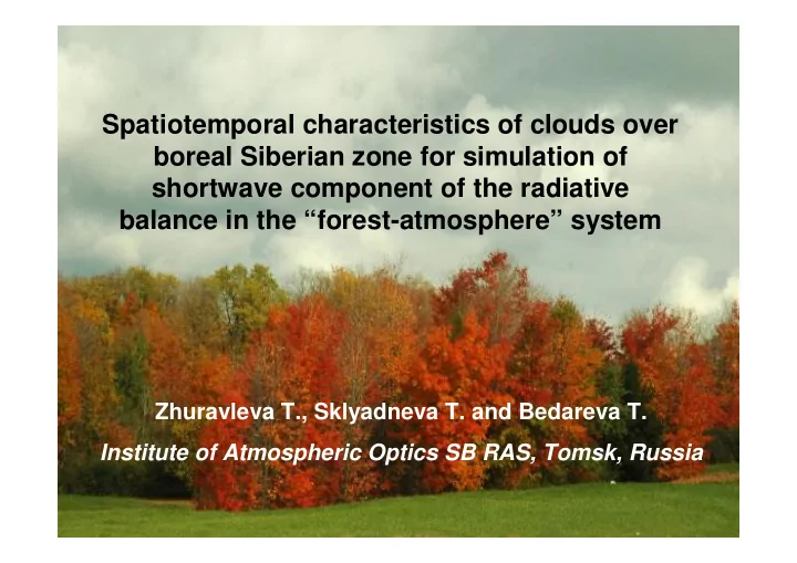
Spatiotemporal characteristics of clouds over boreal Siberian zone for simulation of shortwave component of the radiative balance in the “forest-atmosphere” system Zhuravleva T., Sklyadneva T. and Bedareva T. Institute of Atmospheric Optics SB RAS, Tomsk, Russia
Clouds and climate Cloud radiative forcing CRF = CRW SW + CRF LW , CRF SW = A – A clr , CRF LW = F TOA,clr - F TOA Estimates of annually mean global average values of CRF , W/m 2 Basis Researcher Source CRF LW CRF SW CRF Simple Schneider(1972) 37.5 -65 -27.5 models Cess (1976) 45.5 -44.5 +1 Satellites Ramanathan et ERBE 31 -48 -17 al. (1989) Ardanuy et al. Nimbus 7 24 -51 -27 (1991) 6 climate Cess and Potter Variability {23,55} {-74,- 45} {-34,-2} models (1987) range, January 19 climate Cess et al. (1990) Variability {13,48} {-70,- 33} {-45,-2} models range, July average average= average= =29 -50 -21
Ultimate goal of the work is: on the basis of numerical simulation, to estimate • (i) the radiation budget and (ii) cloud and aerosol radiative forcing in the boreal zone of Siberia to identify the regional features of RB, CRF, and ARF • Purpose of the first stage is: • the development of radiation code • selection of the input atmospheric parameters (cloud characteristics)
Model of solar radiative transfer (IAOT radiation code, Tomsk, Russia) clouds – aerosol – atmospheric gases – underlying surface Radiative characteristics: • fluxes and brightness fields • spectral and integrated characteristics ( ) ( ) ( ) ( ) M ↑ ↓ ↑ ↓ 0.2-5 µ m, M=30 = ∑ F z F z i = i 1 Monte Carlo method Accounting for the molecular absorption: k-distribution technique (HITRAN-04, MT_CKD) )
IAOT radiation code 1. Horizontally homogeneous atmosphere r ω ⊕ Z top H atm ( ) σ σ µ , , g cl , j cl , s , j cl , j top H i p i , T i ( ) ( ) σ σ µ σ ε µ , , g , , , g a , i a , s , i a , i R , i m , i R , i bot H i A s X 0
IAOT radiation code 2. Spatially inhomogeneous clouds: 3D cloud effects Radiative characteristics within one cloud realization Stratocumulus clouds: Moeng et al., 1996: 64 × 64 × 16 (55 m × 55 m × 25 m) 3. Statistical theory of radiative transfer in clouds: average (over cloud realizations) radiative characteristics Poisson model of broken clouds: Analytical averaging of RTE , closed system of equations for first and second intensity moments; algorithms of MC method
Testing of IAOT radiation code Comparison of model calculations and measurement data Spectral fluxes in the cloudy atmosphere Li, Trishchenko, Cribb (Canada), Kiedron, Harrison (USA), Firsov, Zhuravleva RSS 0,4 MOTRAN4 ( Cribb ) 2 *nm) IAOT Data of field experiments: 0,3 Spectral fluxes, Wt/(m overcast one-layer low-level clouds , ARM Southern Great Plains site, Oklahoma, USA, 0,2 1997-1998. 19.10.1997 Cloud layer: 0.58 - 0.85 km Rotating Shadowband LWP =0.008 cm, r ef =7.2 µ m 0,1 Spectroradiometer: 350-1075 2 WVC =1.6 g/cm nm, 512/1024 channels, o ξ 0 =47 direct, diffuse, total radiation 0,0 550 600 800 850 900 950 1000 1050 Wavelength, nm 3D cloud effects: Intercomparison of 3D Radiation Codes
Input parameters Clouds: • optical thickness • single scattering albedo • phase scattering function (asymmetry factor) • cloud fraction • layer’s location (lower and upper boundaries) • cloud horizontal sizes Aerosol: • optical thickness • single scattering albedo • phase scattering function (asymmetry factor) Atmospheric gases: • profiles of temperature, pressure, concentrations Underlying surface: • reflection’s law (Lambert) • surface albedo
Input parameters Cloud characteristics MODIS (collection 5): 2000, April – 2008, … Spatial resolution – 1 degree, time resolution – 1 month • cloud fraction • cloud optical thickness (water and ice phases) • cloud effective radius (water and ice phases) • cloud top pressure • aerosol optical depth (0.55 µ m) • water vapor content (cloudy and clear sky)
Input parameters Software Environment of code development: С ++ Builder 5.0
Input parameters Cloud fraction (Day and Night) January, 2001-2008 July, 2000-2007 N mean =6.8, N min =4.3, N max =8.4 N mean =6.1, N min =3.8, N max =8 68 68 1 Latitude, deg 64 64 0,9 Latitude, deg 60 0,7 60 0,5 56 56 0,3 52 52 60 70 80 90 100 110 120 130 60 70 80 90 100 110 120 130 Longtitude, deg Longtitude, deg Frequency of occurence, % 60 60 Frequency of occurence, % 50 50 40 40 30 30 20 20 10 10 0 0,4 0,5 0,6 0,7 0,8 0,9 0 0,4 0,5 0,6 0,7 0,8 0,9 Cloud fraction Cloud fraction
Input parameters Comparison of surface observations and MODIS data ( ) ( ) ( ) ( ) ( ) sur sat sat sat = + − Mullamaa , 1972 : N N 0 . 05 N 10 N - Surface observations - MODIS o 16'N, 104 o 24'E o 34'N, 69 o 28'E Dem'janskoe, 59 Irkutsk: 52 1,0 1,0 0,8 0,8 0,6 0,6 0,4 0,4 2005 2006 2007 2005 2006 2007 o 26'N,84 o 58'E o 02'N, 92 o 45'E Tomsk, 56 Krasnojarsk: 56 1,0 1,0 0,8 0,8 0,6 0,6 0,4 0,4 2005 2006 2007 2005 2006 2007
Input parameters Cloud optical thickness January, 2001-2008 July, 2000-2007 τ mean =40, τ min =6.7, τ max =100 τ mean =19.2, τ min =13.7, τ max =27.4 68 64 64 30 80 70 25 60 60 60 50 20 40 56 56 30 15 20 10 10 52 52 60 70 80 90 100 110 120 130 60 70 80 90 100 110 120 130 Longtitude, deg Longtitude, deg Frequency of occurence, % Frequency of occurence, % 70 70 60 60 50 50 40 40 30 30 20 20 10 10 0 0 0 10 20 30 40 50 60 70 80 90 100 12 16 20 24 28 Cloud optical thickness Cloud optical thickness
Input parameters Spectral cloud optical characteristics Optical thickness (extinction coefficient), single scattering albedo, phase scattering function (asymmetry factor) 1. Particle size distribution + refractive index => Mie theory 2. Parameterizations of optical characteristics ∞ ∞ ( ) ( ) = 3 2 ∫ ∫ τ =3 LWP /(2 ρ r ef ) , r ef r f r dr r f r dr 0 0 2a. Slingo, Scherker, 1984; Slingo, 1989: 4.2< r ef < 16.6 µ m τ i = LWP ( a i + b i / r ef ); ω i =1- c i - d i r ef ; g i = e i + f i r ef . 2b. Hu and Stamnes, 1993: 2.5< r ef <60 mm σ i = LWC ( a 1, i × r ef b1, i + c 1, i ); ω i =1- a 2, i × r ef b2, i - c 2, i ; g i = a 3 i × r ef b3, i + c 3, i .
Input parameters Effective radius, water phase January, 2001-2008 July, 2000-2007 r mean =11.9, r min =7.7, r max =20.9 µ m r mean =12.9, r min =11.2, r max =14.5 µ m 68 64 64 15 20 14 18 60 60 13 16 14 12 56 56 12 11 10 52 52 10 60 70 80 90 100 110 120 130 60 70 80 90 100 110 120 130 Longtitude, deg Longtitude, deg 70 70 60 60 50 50 40 40 30 30 20 20 10 10 0 0 6 8 10 12 14 16 18 20 22 10 11 12 13 14 15 16 Effective radius, µ m Effective radius, µ m
On calculation of photosynthetically active radiation in estimation of carbon balance parameters of surface ecosystems Atmospheric model Cloud model – statistically homogeneous, based on the Poisson point fluxes on straight lines Aerosol model – continental aerosol (WCP, 1986) Gaseous model – H 2 O, O 2 , O 3 (HITRAN-2000) Underlying surface – Lambertian law Calculation technique: 400-700 nm λ + 3 i 1 ( ) ( ) ( ) ( ) ∑ ∫ = = λ λ ∆ λ = λ − λ = = , , , 100 , 1 , 2 , 3 ; F z F z F z F z d nm i + PAR i i i 1 i = λ i 1 i
Comparison of model calculations and experimental data Input parameters 140 Cloud fraction N : 120 MODIS/TERRA Atmosphere 2 Measurements, W/m 100 monthly Global Product; 80 60 Aspect ratio γ = H / D: 40 γ = γ ( N ) ( Shmetter , 1987 ), 20 H – geometrical thickness, 0 D – mean horizontal cloud size; 0 20 40 60 80 100 120 140 2 Model calculations, W/m Surface albedo: Measured and model-derived conifer, water, snow,ice monthly mean downward PAR for ( Hook , ASTER Spectral library) BOREAS NSA, 2001–2003
Database for fast calculation of mean PAR values for different geographic latitudes, months, surface types, solar zenith angles and cloud fraction East Siberia, 2001, July PAR, W/m 2 Cloud fraction 64 130 64 0,90 125 0,85 120 0,80 115 62 0,75 62 110 0,70 105 0,65 100 0,60 60 60 95 0,55 90 0,50 85 0,45 Latitude, grad Latitude,grad 80 58 0,40 58 75 0,35 70 0,30 56 56 54 54 52 52 50 50 90 92 94 96 98 100 102 104 106 108 90 92 94 96 98 100 102 104 106 108 Longtitude, grad Longtitude, grad
Conclusions 1. The developed radiation code allows us to efficiently calculate the shortwave radiative fluxes at the different levels under conditions of the cloudy and clear-sky atmosphere 2. It is suggested to use as the source of data on the cloud characteristics the data of satellite scanner MODIS (Spatial resolution – 1 degree, time resolution – 1 month) Problems arising in choice of the input parameters: • cloud optical characteristics – testing? • aerosol optical characteristics and testing? • reflection properties of underlying surface and testing?
Thank you for attention!
Recommend
More recommend
Explore More Topics
Stay informed with curated content and fresh updates.
