Space time analysis of extreme values a Gabriel Huerta Department - PowerPoint PPT Presentation
Space time analysis of extreme values a Gabriel Huerta Department of Mathematics and Statistics University of New Mexico Albuquerque, NM, 87131, U.S.A. http://www.stat.unm.edu/ ghuerta 4th EVA conference, Gothenburg, August 15-19 2005 a
Space time analysis of extreme values a Gabriel Huerta Department of Mathematics and Statistics University of New Mexico Albuquerque, NM, 87131, U.S.A. http://www.stat.unm.edu/ ∼ ghuerta 4th EVA conference, Gothenburg, August 15-19 2005 a Joint paper with Bruno Sanso, University of California, Santa Cruz, U.S.A
Summary Points
Summary Points • Models for non-stationary extreme values.
Summary Points • Models for non-stationary extreme values. • Space-time formulation for the GEV distribution.
Summary Points • Models for non-stationary extreme values. • Space-time formulation for the GEV distribution. • Dynamic Linear Model (DLM) framework for temporal components.
Summary Points • Models for non-stationary extreme values. • Space-time formulation for the GEV distribution. • Dynamic Linear Model (DLM) framework for temporal components. • Spatial elements through process convolutions.
Summary Points • Models for non-stationary extreme values. • Space-time formulation for the GEV distribution. • Dynamic Linear Model (DLM) framework for temporal components. • Spatial elements through process convolutions. • Model fitting via customized Markov chain Monte Carlo (MCMC) methods.
Summary Points • Models for non-stationary extreme values. • Space-time formulation for the GEV distribution. • Dynamic Linear Model (DLM) framework for temporal components. • Spatial elements through process convolutions. • Model fitting via customized Markov chain Monte Carlo (MCMC) methods. • Extreme values of ozone levels in Mexico City.
Summary Points • Models for non-stationary extreme values. • Space-time formulation for the GEV distribution. • Dynamic Linear Model (DLM) framework for temporal components. • Spatial elements through process convolutions. • Model fitting via customized Markov chain Monte Carlo (MCMC) methods. • Extreme values of ozone levels in Mexico City. • Extreme values of rainfall in Venezuela.
Figure 1: Daily maximum values of ozone levels. 0.3 Ozone 0.2 0.1 0.0 1990 1992 1994 1996 1998 2000 2002 Time
Extreme Value Modeling
Extreme Value Modeling • The traditional approach is based on the Generalized Ex- treme Value (GEV) distribution function: � � �� − 1 /ξ � � z − µ H ( z ) = exp − 1 + ξ σ +
Extreme Value Modeling • The traditional approach is based on the Generalized Ex- treme Value (GEV) distribution function: � � �� − 1 /ξ � � z − µ H ( z ) = exp − 1 + ξ σ + – −∞ < µ < ∞ ; σ > 0 ; −∞ < ξ < ∞ .
Extreme Value Modeling • The traditional approach is based on the Generalized Ex- treme Value (GEV) distribution function: � � �� − 1 /ξ � � z − µ H ( z ) = exp − 1 + ξ σ + – −∞ < µ < ∞ ; σ > 0 ; −∞ < ξ < ∞ . – + denotes the positive part of the argument.
Extreme Value Modeling • The traditional approach is based on the Generalized Ex- treme Value (GEV) distribution function: � � �� − 1 /ξ � � z − µ H ( z ) = exp − 1 + ξ σ + – −∞ < µ < ∞ ; σ > 0 ; −∞ < ξ < ∞ . – + denotes the positive part of the argument. – ξ > 0 Fr´ echet family; ξ < 0 the Weibull family; ξ → 0 Gumbel family.
• The book by Coles (2001) presents a very clear account of statistical inference using the GEV.
• The book by Coles (2001) presents a very clear account of statistical inference using the GEV. • A Bayesian analysis can be performed by imposing a prior on ( µ, σ, ξ ) as in Coles and Tawn (1996).
• The book by Coles (2001) presents a very clear account of statistical inference using the GEV. • A Bayesian analysis can be performed by imposing a prior on ( µ, σ, ξ ) as in Coles and Tawn (1996). • Alternatively, models for exceedances over a high treshold had been proposed.
• The book by Coles (2001) presents a very clear account of statistical inference using the GEV. • A Bayesian analysis can be performed by imposing a prior on ( µ, σ, ξ ) as in Coles and Tawn (1996). • Alternatively, models for exceedances over a high treshold had been proposed. • This leads into the Generalized Pareto Distributions and Point processes approaches. (Pickands 1971 and 1975).
• The book by Coles (2001) presents a very clear account of statistical inference using the GEV. • A Bayesian analysis can be performed by imposing a prior on ( µ, σ, ξ ) as in Coles and Tawn (1996). • Alternatively, models for exceedances over a high treshold had been proposed. • This leads into the Generalized Pareto Distributions and Point processes approaches. (Pickands 1971 and 1975). • These ideas had been developed into a Bayesian hierarchi- cal modeling framework. Smith et al. (1997); Assuncao et al. (2004); Casson and Coles (1999); Gilleland et. al. (2004).
Extremes for Non-Stationary Data
Extremes for Non-Stationary Data • Coles (2001) mentions several possibilities.
Extremes for Non-Stationary Data • Coles (2001) mentions several possibilities. • Approach: z 1 , z 2 , . . . , z m ; z t ∼ GEV ( µ t , σ, ξ ) .
Extremes for Non-Stationary Data • Coles (2001) mentions several possibilities. • Approach: z 1 , z 2 , . . . , z m ; z t ∼ GEV ( µ t , σ, ξ ) . • Deterministic functions: µ t = β 0 + β 1 t ; µ t = β 0 + β 1 + β 2 t + β 3 t 2 or µ t = β 0 + β 1 X t .
Extremes for Non-Stationary Data • Coles (2001) mentions several possibilities. • Approach: z 1 , z 2 , . . . , z m ; z t ∼ GEV ( µ t , σ, ξ ) . • Deterministic functions: µ t = β 0 + β 1 t ; µ t = β 0 + β 1 + β 2 t + β 3 t 2 or µ t = β 0 + β 1 X t . • Non-stationarity can also be included for the shape and/or scale parameters: σ t = exp ( β 0 + β 1 t ) ; ξ t = β 0 + β 1 t or ξ t = β 0 + β 1 t + β 2 t 2 .
Extremes for Non-Stationary Data • Coles (2001) mentions several possibilities. • Approach: z 1 , z 2 , . . . , z m ; z t ∼ GEV ( µ t , σ, ξ ) . • Deterministic functions: µ t = β 0 + β 1 t ; µ t = β 0 + β 1 + β 2 t + β 3 t 2 or µ t = β 0 + β 1 X t . • Non-stationarity can also be included for the shape and/or scale parameters: σ t = exp ( β 0 + β 1 t ) ; ξ t = β 0 + β 1 t or ξ t = β 0 + β 1 t + β 2 t 2 . • We propose the use of Dynamic Linear Models (DLM) as in West and Harrison (1997) to model the parameter changes in time.
GEV distribution with DLM’s
GEV distribution with DLM’s • For z 1 , z 2 , . . . , z m , z t ∼ GEV ( µ t , σ, ξ ) � � − [1 + ξ ( z t − µ t ) /σ ] − 1 /ξ H t ( z t ) = exp + µ t = θ t + ǫ t ; ǫ t ∼ N (0 , V ) θ t = θ t − 1 + ω t ; ω t ∼ N (0 , τV )
GEV distribution with DLM’s • For z 1 , z 2 , . . . , z m , z t ∼ GEV ( µ t , σ, ξ ) � � − [1 + ξ ( z t − µ t ) /σ ] − 1 /ξ H t ( z t ) = exp + µ t = θ t + ǫ t ; ǫ t ∼ N (0 , V ) θ t = θ t − 1 + ω t ; ω t ∼ N (0 , τV ) • Parameters ( t = 0 ) are assumed apriori independent.
GEV distribution with DLM’s • For z 1 , z 2 , . . . , z m , z t ∼ GEV ( µ t , σ, ξ ) � � − [1 + ξ ( z t − µ t ) /σ ] − 1 /ξ H t ( z t ) = exp + µ t = θ t + ǫ t ; ǫ t ∼ N (0 , V ) θ t = θ t − 1 + ω t ; ω t ∼ N (0 , τV ) • Parameters ( t = 0 ) are assumed apriori independent. • π ( σ ) ∼ LN ( m σ , s σ ) ; π ( ξ ) ∼ N ( m ξ , s ξ ) . • θ 0 ∼ N ( m 0 , C 0 ) ; V ∼ IG ( α v , β v ) ; τ ∼ IG ( α τ , β τ )
GEV distribution with DLM’s • For z 1 , z 2 , . . . , z m , z t ∼ GEV ( µ t , σ, ξ ) � � − [1 + ξ ( z t − µ t ) /σ ] − 1 /ξ H t ( z t ) = exp + µ t = θ t + ǫ t ; ǫ t ∼ N (0 , V ) θ t = θ t − 1 + ω t ; ω t ∼ N (0 , τV ) • Parameters ( t = 0 ) are assumed apriori independent. • π ( σ ) ∼ LN ( m σ , s σ ) ; π ( ξ ) ∼ N ( m ξ , s ξ ) . • θ 0 ∼ N ( m 0 , C 0 ) ; V ∼ IG ( α v , β v ) ; τ ∼ IG ( α τ , β τ ) . • µ t follows a first order polynomial DLM with state vector θ t .
General DLM ( F t , V, G t , W )
General DLM ( F t , V, G t , W ) ′ µ t = F t θ t + ǫ t ; ǫ t ∼ N (0 , V ) θ t = G t θ t − 1 + ω t ; ω t ∼ N (0 , W )
General DLM ( F t , V, G t , W ) ′ µ t = F t θ t + ǫ t ; ǫ t ∼ N (0 , V ) θ t = G t θ t − 1 + ω t ; ω t ∼ N (0 , W ) • θ t is a k × 1 state vector; • F t is a k × 1 regressor vector; • G t is a k × k evolution matrix; • V is an observational variance and • W is a k × k evolution covariance matrix.
Posterior Inference for DLM-GEV models
Posterior Inference for DLM-GEV models • Define Z = ( z 1 , z 2 , . . . , z m ) ; µ = ( µ 1 , µ 2 , . . . , µ m ) and θ = ( θ 1 , θ 2 , . . . , θ m ) .
Posterior Inference for DLM-GEV models • Define Z = ( z 1 , z 2 , . . . , z m ) ; µ = ( µ 1 , µ 2 , . . . , µ m ) and θ = ( θ 1 , θ 2 , . . . , θ m ) . • p ( µ t | z t , σ, θ t , V ); t = 1 , . . . , m is sampled with a Metropolis-Hastings step.
Posterior Inference for DLM-GEV models • Define Z = ( z 1 , z 2 , . . . , z m ) ; µ = ( µ 1 , µ 2 , . . . , µ m ) and θ = ( θ 1 , θ 2 , . . . , θ m ) . • p ( µ t | z t , σ, θ t , V ); t = 1 , . . . , m is sampled with a Metropolis-Hastings step. • p ( σ | Z, µ, ξ ) and p ( ξ | Z, µ, σ ) are also sampled via M-H.
Recommend
More recommend
Explore More Topics
Stay informed with curated content and fresh updates.


