Sorting is removing inversions. In an array sorted by ( ! ) we have [ - PDF document
Sorting is removing inversions. In an array sorted by ( ! ) we have [ ] ! [ ] ( ) i j , 0 i j n A i A j . If the array isnt " ! < < # completely sorted, it will contain inversions . That is, ( % [ ] > [ ] ) i
Sorting is removing ‘inversions’. In an array sorted by ( ! ) we have [ ] ! [ ] ( ) i j , 0 i j n A i A j . If the array isn’t " ! < < # completely sorted, it will contain inversions . That is, ( % [ ] > [ ] ) i j , 0 i j n A i A j . $ ! < < Sorting can be seen as a process of removing those inversions, by exchanging (permuting) elements. Suppose that x<->y is an ‘exchange’ instruction, which swaps the contents of two variables or array elements. Here’s insertion sort again: for (int i=1; i<n; i++) { for (int j=i; j!=0 && A[j-1]>A[j]; j--) A[j-1]<->A[j]; } Each step of the inner loop removes exactly one inversion. Richard Bornat 1 18/9/2007 I2A 98 slides 3 Dept of Computer Science
This program always does n comparisons A[j-1]>A[j] , plus, for each inversion it finds, an exchange A[j-1]<->A[j] and another comparison. In general, for an array of size N containing I inversions, it takes time proportional to N + . I And thus insertion sort is O N ( ) in a sorted array (because I = 0), and ‘runs quickly’ (Weiss) on an ‘almost sorted’ array (one in which I is small). Weiss (p226) shows that the number of inversions in ( an array is at most N N & 1 2, and on average is ) ( ) 1 4. This explains why insertion sort is O N 2 N N & ( ) both in the worst case and on average. Weiss’s argument doesn’t work if the array contains duplicate elements. Why not? Richard Bornat 2 18/9/2007 I2A 98 slides 3 Dept of Computer Science
Shellsort: a better insertion sort. Named for its inventor, Donald Shell. Really. Insertion sort does a fixed amount of work to remove each inversion. Shell sort can remove several inversions with one exchange. ( ) in the worst 32 Its running time is proved to be O N ( ) (Weiss 54 case, and seems on average to be O N ( ) 76 p230). It might even be as good as O N But nobody is quite sure. Really. Richard Bornat 3 18/9/2007 I2A 98 slides 3 Dept of Computer Science
Consider the ‘ h -chains’ ( h ' 1) of A [ 0 .. & n 1 ] : A [ ] 0 , A h A [ ] , [ 2 h ] ,... A [ ] 1 , A h [ 1 ] , A [ 2 h 1 ] ,... + + A [ ] 2 , A h [ 2 ] , A [ 2 h 2 ] ,... + + ... A h [ 1 ] , A [ 2 h 1 ] , A h [ 3 1 ] ,... & & & The chains are disjoint. disjoint : share no elements. Technical language. We can sort them, if we wish, separately. Why should we wish? Well: it is a lot quicker to sort h little h -chains than 2 2 × ( ) = one large array ( h N h N h ); each re-arrangement in a chain has a chance of removing a lot of inversions between the elements moved and elements in other chains. Together these give us the magic. Richard Bornat 4 18/9/2007 I2A 98 slides 3 Dept of Computer Science
We sort the h -chains with large spacing h , then we reduce h a bit and do it again, then reduce again and sort again, ... , then finally sort with h = 1 on the whole array. Here’s a partial description of the algorithm. STARTINGGAP and NEXTGAP are parameters, which I will discuss later: for (int h = STARTINGGAP; h>0; h=NEXTGAP) { for (int i = h; i<n; i++) { for (int j=i; j>=h && A[j]>A[j-h]; j-=h) A[j-h]<->A[j]; } } The elements in A [ 0 .. & h 1 ] are each the first in their chains, so we start with i = . Then each value of i in h h h , 1 , h 2 ,..., n 1 is a position in an h -chain, and + + & we insertion-sort an element into that chain (lines 3 and 4). Richard Bornat 5 18/9/2007 I2A 98 slides 3 Dept of Computer Science
We get different efficiency, depending on we write in place of STARTINGGAP and NEXTGAP . It’s subtle, and we have to rely on experts for information. If you see yourself as a computer science professor one day, this might be a point to start! Try following up the references in Weiss, and try reading some of the proofs for yourself. Weiss (p230) points out that if we write for (int h=n/2; h>0; h=h/2) ( ) then there is a possible worst case which gives O N 2 performance. He then states that if you write a loop which starts with n ÷ 2 and divides by 2 at each step, but adds 1 if ( ) in the worst 32 you get an even answer, you get O N ( ) in the average case. 54 case and O N for (int h=n/2; h>0; h=h/2, h=h-h%2+1) At present there is no proof of the average-case result. It’s an experimental result. If you divide by 2.2 instead of 2, you get even better ( ) – and nobody knows why! The 76 performance – O N algorithm is on p229. Richard Bornat 6 18/9/2007 I2A 98 slides 3 Dept of Computer Science
How can it work so well? An array in which the h -chains are sorted, for some value of h , is h -sorted . So an array might be 5-sorted, or 3-sorted, or 17-sorted, or all the above. Fact about Shellsort: when you take an h -sorted array and j -sort it ( j < ), you finish up with something that h is both j -sorted and h -sorted. I think I can see why this is, but I’m not going to put it on a slide yet. The effect is to produce a final sort which is just insertion sort (because h = 1), which is fast because most of the inversions have already gone. Note that the formulæ STARTINGGAP and NEXTGAP have to be designed to produce a sequence h h , ,..., h 0 which ends with k k & 1 h 0 = , otherwise the sort won’t complete properly. 1 Richard Bornat 7 18/9/2007 I2A 98 slides 3 Dept of Computer Science
The performance of Shellsort. In the next batch of slides there is a health warning about the kind of graphs shown on the next few slides. You have to consider ‘constants of proportionality’ before you can compare different algorithms, not just the magnitude of the formulae in an O ... ( ) judgement. But it’s still interesting to see how the different formulæ behave. 32 (Shellsort worst case) grows much more quickly N than N lg N (we shall soon see some fancy sorting algorithms which run in N lg N time): 35000000 30000000 25000000 20000000 15000000 10000000 5000000 0 0 10000 20000 30000 40000 50000 60000 70000 80000 90000 100000 n lg n n^3/2 Richard Bornat 8 18/9/2007 I2A 98 slides 3 Dept of Computer Science
But you have to go to quite large numbers before 54 (Shellsort average time, N lg N is smaller than N using halving to odd numbers): 1800000 1600000 1400000 1200000 1000000 800000 600000 400000 200000 0 0 10000 20000 30000 40000 50000 60000 70000 80000 90000 100000 n lg n n^7/6 n^5/4 Richard Bornat 9 18/9/2007 I2A 98 slides 3 Dept of Computer Science
54 grows more quickly than N After that point N lg N , so the latter’s advantage grows. 35000000 30000000 25000000 20000000 15000000 10000000 5000000 0 0 100000 200000 300000 400000 500000 600000 700000 800000 900000 1000000 n lg n n^7/6 n^5/4 76 ! But look at N Richard Bornat 10 18/9/2007 I2A 98 slides 3 Dept of Computer Science
76 (Shellsort Even at a value of one hundred million, N average time, using divide by 2.2) hasn’t overtaken N lg N yet: 3000000000 2500000000 2000000000 1500000000 1000000000 500000000 0 0 10000000 20000000 30000000 40000000 50000000 60000000 70000000 80000000 90000000 1E+08 n lg n n^7/6 Richard Bornat 11 18/9/2007 I2A 98 slides 3 Dept of Computer Science
It happens eventually, as it must, somewhere round about half a billion: 35000000000 30000000000 25000000000 20000000000 15000000000 10000000000 5000000000 0 1E+08 2E+08 3E+08 4E+08 5E+08 6E+08 7E+08 8E+08 9E+08 1E+09 0 n lg n n^7/6 What these graphs tell us is that Shellsort may be a serious rival to the N lg N algorithms which we shall consider later. But experiment rules everything. To see which is faster, we shall have to conduct program races. Actually, you shall conduct the races, in the lab. Richard Bornat 12 18/9/2007 I2A 98 slides 3 Dept of Computer Science
Recommend
More recommend
Explore More Topics
Stay informed with curated content and fresh updates.
