Some Uses of CE "Using Consumer Theory to Test Business Cycle - PowerPoint PPT Presentation
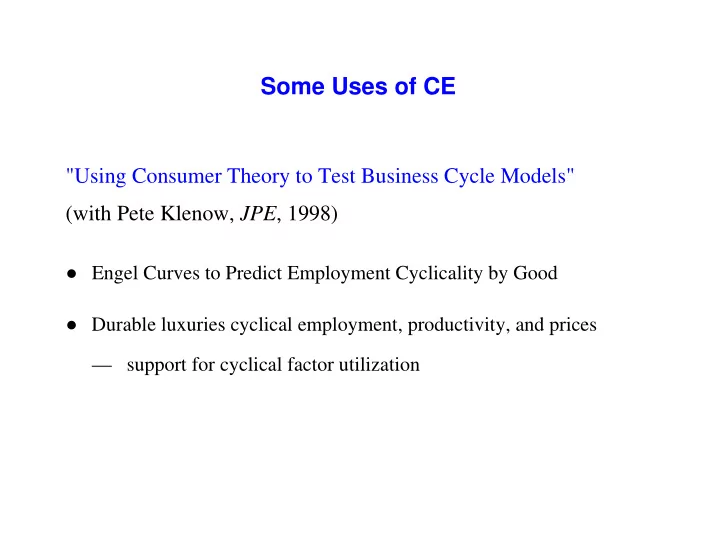
Some Uses of CE "Using Consumer Theory to Test Business Cycle Models" (with Pete Klenow, JPE , 1998) Engel Curves to Predict Employment Cyclicality by Good Durable luxuries cyclical employment, productivity, and prices
Some Uses of CE "Using Consumer Theory to Test Business Cycle Models" (with Pete Klenow, JPE , 1998) ● Engel Curves to Predict Employment Cyclicality by Good ● Durable luxuries cyclical employment, productivity, and prices — support for cyclical factor utilization
"Quantifying Quality Growth" (with Pete Klenow, AER , 2001) ● Estimate Quality Engel Curves for Durables ● Use Quality Engel Curves as instrument for Quality ● Predicts Unit-Price inflation 1980-1996 across goods ● Also Predicts CPI inflation across goods
Figure 3 Quality Engel Curve for CARS 1.0 real price of car purchased (in logs) 0.5 0.0 OLS -0.5 Kernel -1.0 -1.0 -0.5 0.0 0.5 1.0 household real nondurable consumption (in logs)
Figure 4 Quality Engel Curve for VACUUMS 0.3 real price of vacuum purchased (in logs) 0.2 OLS 0.1 0.0 -0.1 Kernel -0.2 -1.0 -0.5 0.0 0.5 1.0 household real nondurable consumption (in logs)
Figure 5 5 1980-1996 Unit Price Inflation 0 -5 corr = .51 -10 0.0 0.2 0.4 0.6 0.8 1.0 1.2 Quality Slope
"Has Consumption Inequality Mirrored Income Inequality?" (with Mark Aguiar, 2010) ● Large increase in income inequality over last 30 years ● Consumption inequality, measured by CE, rose much less — e.g., Slesnick (2001), Krueger and Perri (2006) ● Use budget constraint and CE data on savings to check consistency ● Use Engel curves across goods for alternative measure — Corrects for systematic errors by good or income
Implied Consumption Inequality 0.40 After Tax Income 0.35 0.30 Log Change from 1980-82 0.25 0.20 0.15 0.10 0.05 0.00 1980 1983 1986 1989 1992 1996 1999 2002 2005
Implied Consumption Inequality 0.40 After Tax Income 0.35 0.30 Log Change from 1980-82 0.25 0.20 Reported Expenditure 0.15 0.10 0.05 0.00 1980 1983 1986 1989 1992 1996 1999 2002 2005
Implied Consumption Inequality 0.40 After Tax Income 0.35 0.30 Y-S Log Change from 1980-82 0.25 0.20 Reported Expenditure 0.15 0.10 0.05 0.00 1980 1983 1986 1989 1992 1996 1999 2002 2005
Two Good Example: Food and Entertainment 9 8 Nondurable Entertainment 7 6 ng Spendi 5 ve 4 i at Rel Total 3 Expenditure 2 Food at Home 1 0 1980 1983 1986 1989 1992 1996 1999 2002 2005 YEAR
Implied Consumption Inequality 0.40 After Tax Income 0.35 0.30 Y-S Log Change from 1980-82 0.25 0.20 Reported Expenditure 0.15 0.10 0.05 0.00 1980 1983 1986 1989 1992 1996 1999 2002 2005
Implied Consumption Inequality 0.40 After Tax Income 0.35 Estimated Expenditure 0.30 Y-S Log Change from 1980-82 0.25 0.20 Reported Expenditure 0.15 0.10 0.05 0.00 1980 1983 1986 1989 1992 1996 1999 2002 2005
Description of Data Used ● Panel feature of data — to match expenditures to income — to instrument across surveys to address measurement error ● All available years (including 1972-73) to uncover long-term trends ● Interview files: Family, ITAB, and MTAB files (MTABS for finer disaggregation, for unit prices for durables)
Suggestions for CE Survey and Products For many questions aggregate household consumption is key ● Exploit household budget constraint as check ● Begin with estimate aggregate expenditures — bring records of check, credit spending, estimate currency flow ● Then drop number of questions that generate little expenditure share
For many questions need CE’s short panel — match income/spending, estimate life cycle or allow fixed effects ● Reductions in attrition would be great ● Bring in households only for full cycle ● Make existing years easier to use as panel — e.g., consistent set of ID’s across census changes — perhaps produce panel version
Recommend
More recommend
Explore More Topics
Stay informed with curated content and fresh updates.
