Some remarks on VIX futures and ETNs Marco Avellaneda Courant - PowerPoint PPT Presentation
Gatheral 60, September October 13, 2017 Some remarks on VIX futures and ETNs Marco Avellaneda Courant Institute, New York University Joint work with Andrew Papanicolaou, NYU-Tandon Engineering Outline VIX Time-Series: Stylized
Gatheral 60, September October 13, 2017 Some remarks on VIX futures and ETNs Marco Avellaneda Courant Institute, New York University Joint work with Andrew Papanicolaou, NYU-Tandon Engineering
Outline • VIX Time-Series: Stylized facts/Statistics • VIX Futures: Stylized facts/Statistics • VIX ETNS (VXX, XIV) synthetic (futures, notes) • Modeling the VIX curve and implications to ETN trading/investing
The CBOE S&P500 Implied Volatility Index (VIX) • Inspired by Variance Swap Volatility (Whaley, 90’s) 2 = 2𝑓 𝑠𝑈 ∞ 𝑃𝑈𝑁(𝐿, 𝑈, 𝑇) 𝑒𝐿 𝜏 𝑈 𝐿 2 𝑈 0 Here 𝑃𝑈𝑁(𝐿, 𝑈, 𝑇) represents the value of the OTM (forward) option with strike K, or ATM if S=F. • • In 2000, CBOE created a discrete version of the VSV in which the sum replaces the integral and the maturity is 30 days. Since there are no 30 day options, VIX uses first two maturities* 𝑜 1 , 𝑇 ∆𝐿 𝑃𝑈𝑁 𝐿 𝑗 , 𝑈 2 , 𝑇 ∆𝐿 𝑊𝐽𝑌 = 𝑥 1 𝑃𝑈𝑁 𝐿 𝑗 , 𝑈 2 + 𝑥 2 2 𝐿 𝑗 𝐿 𝑗 𝑗=1 𝑗 * My understanding is that recently they could have added more maturities using weekly options as well.
VIX: Jan 1990 to July 2017
Mode Mean Lehman Bros
VIX Descriptive Statistics VIX Descriptive Stats Mean 19.51195 Standard Error 0.094278 Median 17.63 Mode 11.57 Standard Deviation 7.855663 Sample Variance 61.71144 Kurtosis 7.699637 Skewness 2.1027 Minimum 9.31 Maximum 80.86 • Definitely heavy tails • ``Vol risk premium theory’’ implies long -dated futures prices should be above the average VIX. • This implies that the t ypical futures curve should be upward sloping (contango) since mode<average
Is VIX a stationary process (mean-reverting)? Yes and no… • Augmented Dickey-Fuller test rejects unit root if we consider data since 1990. MATLAB adftest(): DFstat=-3.0357; critical value CV= -1.9416; p-value=0.0031. • Shorter time- windows, which don’t include 2008, do not reject unit root • Non-parametric approach (2-sample KS test) rejects unit root if 2008 is included.
VIX Futures (symbol:VX) Contract notional value = VX × 1,000 • • Tick size= 0.05 (USD 50 dollars) • Settlement price = VIX × 1,000 Monthly settlements, on Wednesday at 8AM, prior to the 3 rd Friday (classical option expiration date) • • Exchange: Chicago Futures Exchange (CBOE) • Cash-settled (obviously) VIX VX3 VX4 VX5 VX1 VX6 VX2 • Each VIX futures covers 30 days of volatility after the settlement date. • Settlement dates are 1 month apart. • Recently, weekly settlements have been added in the first two months.
VIX futures 6:30 PM Thursday Sep 14, 2017 Settlement dates : Sep 20, 2017 Oct 18, 2017 Nov 17, 2017 Dec 19, 2017 Jan 16, 2018 Feb 13, 2018 Mar 20, 2018 April 17, 2018
Inter Constant maturity futures (x-axis: days to maturity) Note: Recently introduced weeklies are illiquid and should not be used to build CMF curve
Partial Backwardation: French election, 1 st round
Term-structures before & after French election Before election (risk-on) After election (risk-off)
VIX futures: Lehman week, and 2 months later
A stylized description of the VIX futures cycle Start here • Markets are ``quiet’’, volatility is low , VIX term structure is in contango (i.e. upward sloping) • Risk on: the possibility of market becoming more risky arises; 30-day S&P implied vols rise • VIX spikes, CMF flattens in the front , then curls up, eventually going into backwardation • Backwardation is usually partial (CMF decreases only for short maturities), but can be total in extreme cases (2008) • Risk-off: uncertainty resolves itself, CMF drops and steepens • Most likely state (contango) is restored End here
Statistics of VIX Futures Curves Constant-maturity futures, 𝑊 𝜐 , linearly interpolating quoted futures prices • 𝜐 = 𝜐 𝑙+1 − 𝜐 𝜐 − 𝜐 𝑙 𝑊 𝑊𝑌 𝑙 (𝑢) + 𝑊𝑌 𝑙+1 (𝑢) 𝑢 𝜐 𝑙+1 − 𝜐 𝑙 𝜐 𝑙+1 − 𝜐 𝑙 𝑊𝑌 𝑙 (t)= kth futures price on date t, 𝑊𝑌 0 = VIX, 𝜐 0 = 0, 𝜐 𝑙 = tenor of kth futures
1 M CMF ~ 65% 5M CMF ~ 35%
PCA: fluctuations from average position • Select standard tenors 𝜐 𝑙 , 𝑙 = 0, 30, 60, 90, 120,150, 180, 210 • Dates: Feb 8 2011 to Dec 15 2016 8 𝜐 𝑙 = 𝑚𝑜𝑊 𝜐 𝑙 + 𝑙 𝑚𝑜𝑊 𝑏 𝑗𝑚 Ψ 𝑚 𝑢 𝑗 𝑚=1 • Slightly different from Alexander and Korovilas (2010) who did the PCA of 1-day log-returns. Eigenvalue % variance expl 1 72 2 18 3 6 4 1 5 to 8 <1
Mode is negative
18.7 % 13.5 %
ETFs/ETNs based on futures • Funds track an ``investable index’’, corresponding to a rolling futures strategy • Fund invests in a basket of futures contracts 𝑂 𝑒𝐽 𝑒𝐺 𝑏 𝑗 = fraction (%) of assets in ith future 𝑗 𝐽 = 𝑠 𝑒𝑢 + 𝑏 𝑗 𝐺 𝑗 𝑗=1 • Normalization of weights for leverage: 𝑂 𝑏 𝑗 = 𝛾, 𝛾 = leverage coefficient 𝑗=1
Average maturity of futures is fixed Assume 𝛾 = 1, let 𝑐 𝑗 = fraction of total number of contracts invested in i th futures: • 𝑜 𝑗 𝐽 𝑏 𝑗 𝑐 𝑗 = 𝑜 𝑘 = . 𝐺 𝑗 • The average maturity 𝜄 is typically fixed, resulting in a rolling strategy. 𝑂 𝑂 𝜄 = 𝑐 𝑗 𝑈 𝑗 − 𝑢 = 𝑐 𝑗 𝜐 𝑗 𝑗=1 𝑗=1
Example 1: VXX (maturity = 1M, long futures, daily rolling) Weights are based on 1-M CMF , no leverage 𝑒𝐽 𝐽 = 𝑠𝑒𝑢 + 𝑐 𝑢 𝑒𝐺 1 + (1 − 𝑐 𝑢 )𝑒𝐺 2 𝑐 𝑢 = 𝑈 2 − 𝑢 − 𝜄 𝑐 𝑢 𝐺 1 + (1 − 𝑐 𝑢 )𝐺 2 𝑈 2 − 𝑈 1 𝜄 = 1 month = 30/360 𝜄 = 𝑐 𝑢 𝐺 Notice that since 𝑊 1 + (1 − 𝑐 𝑢 )𝐺 𝑢 2 𝜄 = 𝑐 𝑢 𝑒𝐺 2 + 𝑐 ′ 𝑢 𝐺 1 − 𝑐 ′ 𝑢 𝐺 𝑒𝑊 1 + (1 − 𝑐 𝑢 )𝑒𝐺 we have 2 𝑢 𝜄 𝑒𝑊 𝜄 = 𝑐 𝑢 𝑒𝐺 1 + (1 − 𝑐 𝑢 )𝑒𝐺 𝐺 2 − 𝐺 𝑒𝑢 𝑢 2 1 Hence + 𝑐 𝑢 𝐺 1 + (1 − 𝑐 𝑢 )𝐺 𝑐 𝑢 𝐺 1 + (1 − 𝑐 𝑢 )𝐺 𝑈 2 − 𝑈 𝑊 2 2 1 𝑢
Dynamic link between Index and CMF equations (long 1M CMF, daily rolling) 𝑒𝐽 𝐽 = 𝑠𝑒𝑢 + 𝑐 𝑢 𝑒𝐺 1 + (1 − 𝑐 𝑢 )𝑒𝐺 2 𝑐 𝑢 𝐺 1 + (1 − 𝑐 𝑢 )𝐺 2 𝜄 = 𝑠 𝑒𝑢 + 𝑒𝑊 𝐺 2 − 𝐺 𝑒𝑢 𝑢 1 𝜄 − 𝑐 𝑢 𝐺 1 + (1 − 𝑐 𝑢 )𝐺 𝑈 2 − 𝑈 𝑊 2 1 𝑢 𝜄 𝜐 Slope of the CMF is 𝑒𝐽 𝐽 = 𝑠 𝑒𝑢 + 𝑒𝑊 𝜖 ln 𝑊 𝑢 𝑢 𝜄 − 𝑒𝑢 the relative drift 𝜖 𝜐 𝑊 𝑢 between index and CMF 𝜐=𝜄
Example 2 : XIV, Short 1-M rolling futures This is a fund that follows a DAILY rolling strategy, sells futures, targets 1-month maturity 𝜄 𝜐 𝑒𝐾 𝐾 = 𝑠 𝑒𝑢 − 𝑒𝑊 𝜖 ln 𝑊 𝑢 𝑢 𝜄 + 𝑒𝑢 𝜄 = 1 month = 30/360 𝜖 𝜐 𝑊 𝑢 𝜐=𝜄 In order to maintain average maturities/leverage, funds must ``reload’’ on futures, which keep tending to spot VIX and then expire. Under contango, long ETNs decay, short ETNs increase.
Stationarity/ergodicity of CMF and consequences Integrating the I- equation for VXX and the corresponding J- equation for XIV (inverse): 𝜐 𝜄 𝑒𝑡 𝑊𝑌𝑌 0 − 𝑓 − 𝑠 𝑢 𝑊𝑌𝑌 𝑢 = 𝑊𝑌𝑌 0 1 − 𝑊 𝑢 𝜖 ln 𝑊 𝑢 𝑡 𝜐 𝑓𝑦𝑞 − 0 𝑊 𝜖𝜐 0 𝜐 𝜄 𝑒𝑡 𝑓 − 𝑠 𝑢 𝑌𝐽𝑊 𝑊 𝑢 𝜖 ln 𝑊 0 𝑡 𝑢 − 𝑌𝐽𝑊 0 = 𝑌𝐽𝑊 𝜐 𝑓𝑦𝑞 − 1 0 0 𝑊 𝜖𝜐 𝑢 𝜄 𝜖 ln 𝑊 𝑡 Proposition: If VIX is stationary and ergodic, and 𝐹 > 0, static buy-and-hold XIV or 𝜖𝜐 short-and-hold VXX produce sure profits in the long run, with probability 1.
All data, split adjusted VXX underwent five 4:1 reverse splits since inception Huge volume Flash crash US Gov downgrade Feb 2009
Taking a closer look, last 2 1/2 years Note: borrowing costs for VXX are approximately 3% per annum This means that we still have profitability for shorts after borrowing Costs. ukraine war yuan devaluation brexit trump korea
korea le pen china trump brexit
Modeling CMF curve dynamics • VIX ETNs are exposed to (i) volatility of VIX (ii) slope of the CMF curve • We propose a stochastic model and estimate it. • 1-factor model is not sufficient to capture observed ``partial backwardation’’ and ``bursts’’ of volatility • Parsimony suggests a 2-factor model • Assume mean-reversion to investigate the stationarity assumptions • Sacrifice other ``stylized facts’’ (fancy vol -of-vol) to obtain analytically tractable formulas.
`Classic’ log -normal 2-factor model for VIX 𝑊𝐽𝑌 𝑢 = 𝑓𝑦𝑞 𝑌 1 𝑢 + 𝑌 2 𝑢 𝑒𝑌 1 = 𝜏 1 𝑒𝑋 1 + 𝑙 1 𝜈 1 − 𝑌 1 𝑒𝑢 𝑒𝑌 2 = 𝜏 2 𝑒𝑋 2 + 𝑙 2 𝜈 2 − 𝑌 2 𝑒𝑢 𝑒𝑋 1 𝑒𝑋 2 = 𝜍 𝑒𝑢 𝑌 1 = factor driving mostly VIX or short-term futures fluctuations (slow) 𝑌 2 = factor driving mostly CMF slope fluctuations (fast) These factors should be positively correlated.
Recommend
More recommend
Explore More Topics
Stay informed with curated content and fresh updates.
