Some recent methods in non-rigid shape matching, with and without - PowerPoint PPT Presentation
Some recent methods in non-rigid shape matching, with and without learning GAMES 2019 webinar Maks Ovsjanikov Based on joint work with: E. Corman, Michael Bronstein, Emanuele Rodol, Justin Solomon, Adrien Butscher, Mirela Ben-Chen, Leonidas
Some recent methods in non-rigid shape matching, with and without learning GAMES 2019 webinar Maks Ovsjanikov Based on joint work with: E. Corman, Michael Bronstein, Emanuele Rodolà, Justin Solomon, Adrien Butscher, Mirela Ben-Chen, Leonidas Guibas, Frederic Chazal ….
My Background • 2005 – 2010: PhD from Stanford University (advisor Leonidas Guibas). • 2011: engineer at Google Inc. • Since 2012 Professor in the Computer Science Department at Ecole Polytechnique in France.
University • Ecole Polytechnique: located very near Paris. Ranked 2 nd best small university in the world in 2019. • • Est. 1794. Students and professors such as Ampère, Cauchy, Fourier, Hermite, Lagrange, Monge, Poincaré, Poisson… • Very international campus.
Our group • Currently 5 PhD students and 2 PostDocs. • Part of the larger STREAM team dedicated to visual computing with 3 other professors. • Many international collaborations: Stanford, MIT, UCL, KAUST, Univ. Toronto, Univ. Rome, etc. • Funding for PhD students and postdocs !
General Overview Overall Objective : Create tools for computing and analyzing mappings between geometric objects.
Talk Overview [Related] Course Website: http://www.lix.polytechnique.fr/~maks/fmaps_SIG17_course/ or http://bit.do/fmaps2017 Course Notes: Linked from the website. Or use http://bit.do/fmaps2017_notes Attention: (significantly) more material than in the lectures Sample Code: See Sample Code link on the website. Demo code for basic operations. 6
Talk Overview Motivation and Problem Taxonomy Rigid Matching: ICP Functional Map representation, properties Basic pipeline for non-rigid matching Recent extensions, improvements Open problems, Q&A
What is a Shape? Continuous: a surface embedded in 3D. Discrete: a graph embedded in 3D (triangle mesh). Common assumptions: • Connected. • Manifold. • Without Boundary.
What is a Shape? Continuous: a surface embedded in 3D. Discrete: a graph embedded in 3D (triangle mesh). 5k – 200k triangles Shapes from the FAUST, SCAPE, and TOSCA datasets
Overall Goal Given two shapes, find correspondences between them.
Overall Goal Given two shapes, find correspondences between them. Finding the best map between a pair of shapes.
Problem Taxonomy Local vs. Global refinement (e.g. ICP) | alignment (search) . . Rigid vs. Deformable rotation, translation | general deformation. Semi vs. Fully Automatic given landmarks | a priori model Learning-Based vs. Direct known examples | unseen data
Problem Taxonomy Local vs. Global refinement (e.g. ICP) | alignment (search) . . Rigid vs. Deformable rotation, translation | general deformation. Semi vs. Fully Automatic given landmarks | a priori model Learning-Based vs. Direct known examples | unseen data
Why Shape Matching? Given a correspondence, we can transfer: texture and parametrization segmentation and labels deformation Sumner et al. ‘04. Other applications: shape interpolation, reconstruction ... 14
Rigid Shape Matching • Given a pair of shapes, find the optimal Rigid Alignment between them. • The unknowns are the rotation/translation parameters of the source onto the target shape.
Iterative Closest Point (ICP) • Classical approach: iterate between finding correspondences and finding the transformation: Besl, McKay (1992). "A Method for Registration of 3-D Shapes". example in 2D N M Given a pair of shapes, and , iterate: N M 1. For each find nearest neighbor . y i ∈ N x i ∈ M 2. Find optimal transformation minimizing: � ∥ Rx i + t − y i ∥ 2 arg min 2 R,t i
Iterative Closest Point • Classical approach: iterate between finding correspondences and finding the transformation: N M Given a pair of shapes, and , iterate: N M 1. For each find nearest neighbor . y i ∈ N x i ∈ M 2. Find optimal transformation minimizing: � ∥ Rx i + t − y i ∥ 2 arg min 2 R,t i
Iterative Closest Point • Classical approach: iterate between finding correspondences and finding the transformation: N M Given a pair of shapes, and , iterate: N M 1. For each find nearest neighbor . y i ∈ N x i ∈ M 2. Find optimal transformation minimizing: � ∥ Rx i + t − y i ∥ 2 arg min 2 R,t i
Iterative Closest Point • Classical approach: iterate between finding correspondences and finding the transformation: N M Given a pair of shapes, and , iterate: N M 1. For each find nearest neighbor . y i ∈ N x i ∈ M 2. Find optimal transformation minimizing: � ∥ Rx i + t − y i ∥ 2 arg min 2 R,t i
Iterative Closest Point • Classical approach: iterate between finding correspondences and finding the transformation: N M Given a pair of shapes, and , iterate: N M 1. For each find nearest neighbor . y i ∈ N x i ∈ M 2. Find optimal transformation minimizing: � ∥ Rx i + t − y i ∥ 2 arg min 2 R,t i
Iterative Closest Point • Classical approach: iterate between finding correspondences and finding the transformation: N M 1. Finding nearest neighbors: can be done with space- partitioning data structures (e.g., KD-tree). 2. Finding the optimal transformation minimizing: � ∥ Rx i + t − y i ∥ 2 arg min 2 R,t i Arun et al., Least- Can be done efficiently via SVD decomposition. Squares Fitting of Two 3-D Point Sets
Non-Rigid Shape Matching Unlike rigid matching with rotation/translation, there is no compact representation to optimize for in non-rigid matching. 22
Non-Rigid Shape Matching Main Questions: What does it mean for a correspondence to be “good”? How to compute it efficiently in practice? 23
Isometric Shape Matching Deformation Model: Good maps must preserve geodesic distances. N d N ( T ( x ) , T ( y )) d M ( x, y ) M Geodesic: length of shortest path lying entirely on the surface. 24
Isometric Shape Matching Approach: N d N ( T ( x ) , T ( y )) d M ( x, y ) M Find the point mapping by minimizing the distance distortion: ∥ d M ( x, y ) − d N ( T ( x ) , T ( y )) ∥ � T opt = arg min T x,y The unknowns are point correspondences.
Isometric Shape Matching Approach: N d N ( T ( x ) , T ( y )) d M ( x, y ) M Find the point mapping by minimizing the distance distortion: ∥ d M ( x, y ) − d N ( T ( x ) , T ( y )) ∥ � T opt = arg min T x,y Problem: The space of possible solutions is highly non-linear, non-convex.
Functional Map Representation We would like to define a representation of shape maps that is more amenable to direct optimization. 1. A compact representation for “natural” maps. 2. Inherently global and multi-scale. 3. Handles uncertainty and ambiguity gracefully. 4. Allows efficient manipulations (averaging, composition). 5. Leads to simple (linear) optimization problems. 27
Functional Approach to Mappings Given two shapes and a pointwise map T : N → M N T M The map induces a functional correspondence: T T F ( f ) = g, where g = f ◦ T 28 Functional maps: a flexible representation of maps between shapes, O., Ben-Chen, Solomon, Butscher, Guibas , SIGGRAPH 2012
Functional Approach to Mappings Given two shapes and a pointwise map T : N → M T F ( f ) = g : N → R T F f : M → R The map induces a functional correspondence: T T F ( f ) = g, where g = f ◦ T 29 Functional maps: a flexible representation of maps between shapes, O., Ben-Chen, Solomon, Butscher, Guibas , SIGGRAPH 2012
Functional Approach to Mappings Given two shapes and a pointwise map T : N → M T F ( f ) = g : N → R T F f : M → R The map induces a functional correspondence: T T F ( f ) = g, where g = f ◦ T 30 Functional maps: a flexible representation of maps between shapes, O., Ben-Chen, Solomon, Butscher, Guibas , SIGGRAPH 2012
Functional Approach to Mappings Given two shapes and a pointwise map T : N → M T F ( f ) = g : N → R T F f : M → R The induced functional correspondence is linear: T F ( α 1 f 1 + α 2 f 2 ) = α 1 T F ( f 1 ) + α 2 T F ( f 2 ) 31
Functional Map Representation Given two shapes and a pointwise map T : N → M T F ( f ) = g : N → R T F f : M → R The induced functional correspondence is complete. 32
Observation Assume that both: f ∈ L 2 ( M ) , g ∈ L 2 ( N ) g : N → R T F f : M → R N M Express both and in terms of basis functions: f T F ( f ) � a i φ M � b j φ N f = g = T F ( f ) = i j i j Since is linear, there is a linear transformation from to . { a i } { b j } T F
Functional Map Representation Choice of Basis: Eigenfunctions of the Laplace-Beltrami operator: ∆ φ i = λ i φ i ∆ ( f ) = − div ∇ ( f ) Generalization of Fourier bases to surfaces. Ordered by eigenvalues and provide a natural notion of scale . 34 λ 0 = 0 λ 1 = 2 . 6 λ 2 = 3 . 4 λ 3 = 5 . 1 λ 4 = 7 . 6
Functional Map Representation Choice of Basis: Eigenfunctions of the Laplace-Beltrami operator: ∆ φ i = λ i φ i Generalization of Fourier bases to surfaces. Form an orthonormal basis for . L 2 ( M ) Ordered by eigenvalues and provide a natural notion of scale . Can be computed efficiently, with a sparse matrix eigensolver. 35
Recommend
More recommend
Explore More Topics
Stay informed with curated content and fresh updates.
