SLIDE 1 Some motivating facts
1 / 31
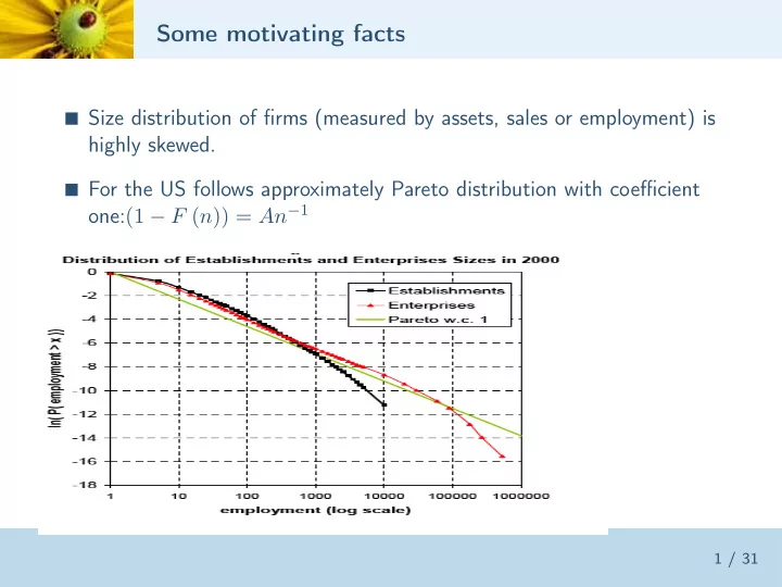
Size distribution of firms (measured by assets, sales or employment) is
highly skewed.
For the US follows approximately Pareto distribution with coefficient
SLIDE 2 more facts
2 / 31
Firm size is persistent but the variance of innovations is quite large. Gross realocation of employment across firms exceeds in several orders of
magnitude net reallocation.
Variance of growth rates declines with size and age. Firm size increases with age. There is considerable degree of entry/exit into narrowly defined
- industries. Small and young firms have higher exit rates.
Most firm level changes in employment correspond to idiosyncratic
shocks, i.e. not explained by aggregate, geographic or industry variables.
SLIDE 3 A simplified Lucas model
3 / 31
Collection of firms i = 1, ..., M Technology yi = einη
i where η < 1
Fixed endowment of labor N Competitive equilibrium {w, ni}maximizing profits and market clearing. n (ei, w) labor demand and n (ei, w) = N Solves planner problem:
maxni
i
SLIDE 4 Equilibrium
4 / 31
Employment:
ni = ae
1 1−η
i
a
1 1−η
i
= N yi = aηeie
η 1−η
i
= aηe
1 1−η
i
Remark yi/ni is the same for all firms! Solving for w and substituting:
y =
yi = aη e
1 1−η
i
=
1 1−η
i
1−η N η
SLIDE 5 The Aggregate Production function
5 / 31
y =
1 1−η
i
1−η N η =
1 1−η
i
1−η M1−ηN η
Cobb Douglass in M, N with TFP equal to geometric average of firm
shocks.
M is like a capital stock, sometimes called "organization capital" Intangible?
SLIDE 6 Multiple inputs
6 / 31
Results generalize to multiple inputs (Lucas 1978) Let f (x) be homogenous of degree one and
yi = ei (f (x))η
aggregate endowment vector X Aggregate production function:
y =
1 1−η
i
1−η M1−ηf (X)η
SLIDE 7 Large number of firms
7 / 31
Let F (e) denote the cdf for shocks. Suppose M is the mass of firms (quantity of organization capital)
y =
1 1−η
1−η M1−ηN η
Special case: F = 1 −
emin
e
α Pareto distribution Ee
1 1−η =
αemin α −
1 1−η
e
1 1−β −α
min
"Tail condition": defined only when α >
1 1−η
SLIDE 8 Endogenizing entry
8 / 31
Technology for creating firms (organization capital) takes ce workers. Entrants draw ei independently from same distribution Planner’s problem:
maxM,L
1 1−η
1−η M1−ηLη subject to : ceM + L ≤ N
solution: L = ηN and M = (1 − η) N/ce
y =
1 1−η
ce 1−η (1 − η)1−η ηη N
Constant returns to scale in aggregate Productivity negatively related to entry cost.
SLIDE 9 Connection to monopolistic competition
9 / 31
Dixit-Stiglitz (1977), Melitz (2003) Continuum of goods: y =
´ yη
i di
1
η
Linear techology yi = eη
i ni
Constant markup pi = 1
η (w/eη i )
yη
i ∝ e
1 1−η
i
and so is ni y =
1 1−η
i
1−η
η
M
1−η η N
yη =
1 1−η
i
1−η M1−ηN η
With endogenous entry get same M.
SLIDE 10
General or partial equilibrium
10 / 31
Partial equilibrium:
Aggregate demand D (p∗) Cost function c (e, q), supply function s (e, p) Entry cost ce Solve for unique p∗that makes expected profits = ce Find MEes (e, p∗) = D (p∗)
Correspondence (w = 1),
c (e, q) = f −1 (q/e) p∗ = 1/w∗
SLIDE 11
Firm dynamics - motivation
11 / 31
Lots of evidence that firms’ size is not constant
Five year AR1 of firm ln employment US manufacturing, persistence
0.92 and large variance of innovation.
Firm size distribution stochastically increases with age.
average entrant 35% size of average incumbent
SLIDE 12 Firm dynamics - simple model
12 / 31
entrants draw independently initial shocks from same distribution firm productivity evolves according to MP F (et+1|et) Repeated application generates probability distributions ˜
µs for firms of age s.
exogenous death/exit rate 1 − δ.
Mt = δtm0 + δt−1m1 + ... + δmt−1 + mt µt = M −1
t
µ0 + δmt−1˜ µ1 + ... + δtm0˜ µt
= ˆ e
1 1−η dµt (e)
1−η M1−η
t
Lη
t
SLIDE 13 Competitive equilibrium
13 / 31
Given sequence of wages w = {wt}∞
t=0
vt (e; w) = maxnenη − wtn + βδEvt+1
t
= E0vt (e; w) − wtce Definition 1. A competitive equilibrium is a sequence {mt, nt (e) , vt} and wages {wt} that satisfy the following conditions:
- 1. Employment decisions are optimal given wages
- 2. value functions are as defined above
- 3. ve
t ≤ 0 and mtve t = 0
´ nt (e) µt (de) = N.
SLIDE 14
Planners problem
14 / 31
Objective:
maxmt,Lt ∞
t=0βt ´
e
1 1−η dµt (e)
1−η M1−η
t
Lη
t
subject to : Mt = δtm0 + δt−1m1 + ... + mt L + cemt = N
Unique solution:
Objective strictly concave Constraints linear
SLIDE 15 Stationary equilibrium
15 / 31
Analogous to steady state (or balanced growth path) Entry flow mt = m for all t. This implies M =
m 1−δ and µ = (1 − δ) ∞ s=0 δs˜
µs
Value function:
v (e) = maxnenη − wn + βδ ˆ v
F
´ n (e, w) dµ (e) + mce = N
Stationary equilibrium is unique. Steady state productivity proportional to:
1 1−η
ce
1−η
SLIDE 16 Costs of entry and TFP
16 / 31
Cross-country regression (Moscoso-Boedo and Mukoyama, 2010) Calculate regulatory costs of creating business measured in units of
annual labor κ
Lowest US κ = 0.3, highest Liberia κ = 616.8, 29 countries with κ < 1
and 31 with κ > 10.
7 6 5 4 3 2 1 1 2 1 1 2 3 4 5 6 Log (GNI p cap relative to US) log() Entry Cost
SLIDE 17 Effects of entry costs in the model
17 / 31
From our previous derivations:
y =
1 1−η
ce + κ 1−η (1 − η)1−η ηη N d ln y/d ln (c + κ) = − (1 − η)
Effects of distortions to entry costs depend on the degree of decreasing
returns
usually take η = 0.85, so d ln y/d ln κ = −0.15 Back of the envelope (Moscoso-Boedo and Mukoyama)
baseline ce = 36. Compare κ = 10 and κ = 100 to κ = 0 κ = 10 → TFP = 0.9, κ = 100 → TFP = 0.6
Sizeable but far from observed differences in TFP.
SLIDE 18
Firm dynamics
18 / 31
Stylized facts:
Small firms grow faster (conditional on survival) Size of firms very persistent (close to random walk) Large firms have lower variance of growth rates Size distribution of firms stochastically increasing in age Exit rates decline with age
Last one cannot be explained in this model that assumes a constant exit
rate
Others depend on assumptions on the distribution F and the initial
distribution of firms shocks, call it G.
SLIDE 19
Age-increasing size distribution
19 / 31
Assumption 1. (FOSD) F (e, e) decreasing in e.
Sequence ˜
µs obtained recursively as ˜ µs+1 ([0, e]) = ´ F ([0, e], e) d˜ µs(e) Assumption 2. F ◦G G (F increases G): ´ F ([0, e], e) dG (e) < G ([0, e])
Persistence and F ◦ G G implies ˜
µs is increasing sequence (in FOSD)
SLIDE 20 Endogenous exit and selection
20 / 31
Firm exit endogenous Need a reason for exiting: fixed costs, opportunity costs Assume fixed cost f denominated in units of labor
v (e; w) = max
ˆ v
- e; w
- F
- de, e
- Decision rules n (e, w) and exit set E (w) .
Proposition 1. (i)v (e; w) strictly decreasing in w if nonzero. (ii)Under (FOSD) v (e; w) strictly increasing in e if nonzero and exit set is threshold e (w) .
Value of entry: ve (w) =
´ v (e; w) dG (e) − ce
SLIDE 21
The invariant measure of firms
21 / 31
Timing: 1) entry; 2) shocks realized, 3) exit; 4) production Entrants: m mass: measure mG Incumbents (before exit): µI (−∞, e) =
´ F (e, e0) µ (de0)
New measure of firms (e ≥ e∗)
Tµ (−∞, e) = m [G (e) − G (e∗)] + µI (e∗, e) = m [G (e) − G (e∗)] + ˆ [F (e, e0) − F (e∗, e0)] µ (de0)
Invariant measure: µ = Tµ
SLIDE 22 Unique invariant measure
22 / 31
Invariant measure as a weighted sum of measure of different cohorts. Let αn be the probability of surviving up to n periods
µ = m
∞
αn˜ µn
Necessary and Sufficient conditoin for existence :
∞
αn < ∞
Integrating by parts: finite expected lifetime
∞
αn =
∞
n (αn+1 − αn) < ∞
SLIDE 23 Stationary equilibrium: definition
23 / 31
{µ, e∗, m, w}
- 1. ve (w) ≤ 0 and ve (w) m = 0
- 2. e∗ is optimal exit rule
- 3. N =
´ (f + n (e, w)) dµ + mce
- 4. µ is an invariant measure
Equilibrium with entry and exit
m > 0 m (1 − G (e∗)) =
´ F (e∗, e) µ (ds)
ve (w∗) = 0 unique
SLIDE 24
Partial equilibrium
24 / 31
Inverse demand p = D (Q) Firms profit and supply function: π (e, p) and q (e, p), strictly increasing
in e and p
Cost of entry ce (fixed costs already included in π (e, p) function) Unique stationary equilibrium {µ, e∗, m, p}
SLIDE 25
Some properties
25 / 31
Size and Age
In the data size distribution stochastically incerases with age In model, depends on properties of F and G Sufficient condtitions:
F (e2, e) 1 − F (e1, e) decreasing in s for all (e, e1) F increases G
Firm growth: depends on properties of F
SLIDE 26
Rate of turnover
26 / 31
Rate of turnover (entry/exit)
m µ (E) = m λ ∞
n=0 αn˜
µn = 1/E (n)
E (n) decreases with e∗ (turnover increases) e∗ increases with w (decreases with p) Higher cost of entry ce, decrease w(increase p), decreases turnover
SLIDE 27 Turnover and Sunk Costs
27 / 31
Indirect measures of sunk costs
Average size of firms Number of firms
Cross industry regression. Dependent: Rate of Entry
Variable Estimate t Intercept
Log Avg Size
Log Num Firms 0.14 12.6
SLIDE 28 Selection and Productivity
28 / 31
Productivity determined by stochastic process (G, F) and exit threshold
Formulas for homogeneous case y =
1 1−η
1−η M1−ηLη L = N − mce − Mf M = m
αn (e∗) Ee
1 1−η =
´
e∗ e
1 1−η dµ
M
Selection effect: Ee
1 1−η increases with threshold e∗so decreases with ce.
Other effects (possibly M decreases), but total productivity must
decrease in ce.
SLIDE 29
Selection and productivity: analysis
29 / 31
No scale effects: Increasing N does not change e∗ and just increases
proportionally m and M.
Aggregate productivity shocks neutral
Changes wage proportionally Does not change employment, exit or entry decisions. Just scales up total output
Aggregate productivity shock that is complementary to e
Increases relative size of larger (higher e) firms Increases exit threshold e∗ (selection effect)
SLIDE 30 Identifying stochastic process
30 / 31
Hopenhayn and Rogerson (JPE 1993) Production function: f (s, n) = snα Let p denote output price (labor as numeraire) ln st+1 = ρ ln st + εt+1, where εt ∼ N
ε, σ2
ε
- First order conditions for employment:ln αp + ln st = (1 − α) ln nt
implies: ln nt+1 = (1 − α)−1 ln st+1 + ln αp = (1 − α)−1 (ρ ln st + εt+1) + ln αp = (1 − α)−1 {(1 − α) ρ ln nt + ρ ln αp + εt+1} + ln αp = A + ρ ln nt + (1 − α)−1 εt+1
ρ and σ identified from AR1 parameters for ln firm size
SLIDE 31
more calibration
31 / 31
The initial distribution determined by distribution of entrants sizes more parameters to determine: cf, ce and the mean ¯
ε.
Data to use: rate of turnover, mean size, age distribution.