Solving the steady state diffusion equation with uncertainty - PowerPoint PPT Presentation
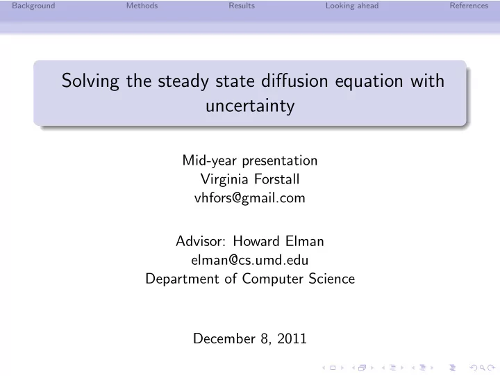
Background Methods Results Looking ahead References Solving the steady state diffusion equation with uncertainty Mid-year presentation Virginia Forstall vhfors@gmail.com Advisor: Howard Elman elman@cs.umd.edu Department of Computer
Background Methods Results Looking ahead References Solving the steady state diffusion equation with uncertainty Mid-year presentation Virginia Forstall vhfors@gmail.com Advisor: Howard Elman elman@cs.umd.edu Department of Computer Science December 8, 2011
Background Methods Results Looking ahead References Problem The equation to be solved is −∇ · ( k ( x , ω ) ∇ u ) = f ( x ) , (1) where k = e a ( x ,ω ) .
Background Methods Results Looking ahead References Problem The equation to be solved is −∇ · ( k ( x , ω ) ∇ u ) = f ( x ) , (1) where k = e a ( x ,ω ) . Assume a bounded spatial domain D ⊂ R 2 .
Background Methods Results Looking ahead References Problem The equation to be solved is −∇ · ( k ( x , ω ) ∇ u ) = f ( x ) , (1) where k = e a ( x ,ω ) . Assume a bounded spatial domain D ⊂ R 2 . The boundary conditions are deterministic.
Background Methods Results Looking ahead References Problem The equation to be solved is −∇ · ( k ( x , ω ) ∇ u ) = f ( x ) , (1) where k = e a ( x ,ω ) . Assume a bounded spatial domain D ⊂ R 2 . The boundary conditions are deterministic. u ( x , ω ) = g ( x ) on ∂ D D ∂ u ∂ n = 0 on ∂ D n .
Background Methods Results Looking ahead References Outline of approach Algorithm
Background Methods Results Looking ahead References Outline of approach Algorithm 1 Approximate the random field using the Karhunen-Lo´ eve expansion.
Background Methods Results Looking ahead References Outline of approach Algorithm 1 Approximate the random field using the Karhunen-Lo´ eve expansion. 2 Solve the PDE using either the stochastic collocation method or stochastic Galerkin method.
Background Methods Results Looking ahead References Outline of approach Algorithm 1 Approximate the random field using the Karhunen-Lo´ eve expansion. 2 Solve the PDE using either the stochastic collocation method or stochastic Galerkin method. Validation Compare the moments of this solution to the moments obtained from solving the equation using the Monte-Carlo method.
Background Methods Results Looking ahead References Karhunen-Lo´ eve expansion The expansion is � � ∞ a ( x , � ξ ) = µ ( x ) + λ s f s ( x ) ξ s . (2) s =1
Background Methods Results Looking ahead References Karhunen-Lo´ eve expansion The expansion is � � ∞ a ( x , � ξ ) = µ ( x ) + λ s f s ( x ) ξ s . (2) s =1 µ ( x ) is the mean of the random field.
Background Methods Results Looking ahead References Karhunen-Lo´ eve expansion The expansion is � � ∞ a ( x , � ξ ) = µ ( x ) + λ s f s ( x ) ξ s . (2) s =1 µ ( x ) is the mean of the random field. The random variables ξ s are uncorrelated.
Background Methods Results Looking ahead References Karhunen-Lo´ eve expansion The expansion is � � ∞ a ( x , � ξ ) = µ ( x ) + λ s f s ( x ) ξ s . (2) s =1 µ ( x ) is the mean of the random field. The random variables ξ s are uncorrelated. The λ s and f s ( x ) are eigenpairs which satisfy � ( C f )( x ) = C ( x , y ) f ( y ) dy = λ f ( x ) , (3) D where C ( x , y ) is the covariance function of the random field.
Background Methods Results Looking ahead References Covariance matrix The covariance matrix for a finite set of points x i in the spatial domain is � C ( x i , x j ) = ( a ( x i , ω ) − µ ( x i ))( a ( x j , ω ) − µ ( x j )) dP ( ω ) , (4) Ω where � µ ( x ) = a ( x , ω ) dP ( ω ) . (5) Ω
Background Methods Results Looking ahead References Covariance matrix The covariance matrix for a finite set of points x i in the spatial domain is � C ( x i , x j ) = ( a ( x i , ω ) − µ ( x i ))( a ( x j , ω ) − µ ( x j )) dP ( ω ) , (4) Ω where � µ ( x ) = a ( x , ω ) dP ( ω ) . (5) Ω Denote the approximation to this matrix C ij = C ( x i , x j ) . (6)
Background Methods Results Looking ahead References Covariance matrix The eigenpairs of the covariance matrix are related to the eigenpairs of the random field.
Background Methods Results Looking ahead References Covariance matrix The eigenpairs of the covariance matrix are related to the eigenpairs of the random field. This is found by taking a discrete approximation to the continuous eigenvalue problem in Equation 3.
Background Methods Results Looking ahead References Covariance matrix The eigenpairs of the covariance matrix are related to the eigenpairs of the random field. This is found by taking a discrete approximation to the continuous eigenvalue problem in Equation 3. For a one-dimensional domain with uniform interval size h , the discretization of this problem is hCV = Λ V . (7)
Background Methods Results Looking ahead References Covariance matrix The eigenpairs of the covariance matrix are related to the eigenpairs of the random field. This is found by taking a discrete approximation to the continuous eigenvalue problem in Equation 3. For a one-dimensional domain with uniform interval size h , the discretization of this problem is hCV = Λ V . (7) For a uniform two-dimensional domain with interval sizes h x and h y , the problem to solve is h x h y CV = Λ V . (8)
Background Methods Results Looking ahead References Covariance matrix When the covariance function for a random field is known, the covariance matrix is constructed by evaluating the function at each pair of points.
Background Methods Results Looking ahead References Covariance matrix When the covariance function for a random field is known, the covariance matrix is constructed by evaluating the function at each pair of points. Otherwise, n samples can be taken at each spatial point to form the sample covariance matrix, � C . n � C ij = 1 � ( a ( x i , ξ k ) − ˆ µ i )( a ( x j , ξ k ) − ˆ µ j ) (9) n k =1 � n µ i = 1 ˆ a ( x i , ξ k ) . (10) n k =1
Background Methods Results Looking ahead References Sample covariance matrix We are interested in the eigenpairs of ˆ C , but do not need to construct the entire matrix.
Background Methods Results Looking ahead References Sample covariance matrix We are interested in the eigenpairs of ˆ C , but do not need to construct the entire matrix. Define a matrix: B ik = a ( x i , ω k ) − ˆ µ i (11)
Background Methods Results Looking ahead References Sample covariance matrix We are interested in the eigenpairs of ˆ C , but do not need to construct the entire matrix. Define a matrix: B ik = a ( x i , ω k ) − ˆ µ i (11) Then the sample covariance matrix can be written as C = 1 nBB T . � (12)
Background Methods Results Looking ahead References Sample covariance matrix Consider the singular value decomposition of B = U Σ V T .
Background Methods Results Looking ahead References Sample covariance matrix Consider the singular value decomposition of B = U Σ V T . The eigenvalues of � C will be 1 n Σ 2 . The eigenvectors of � C will be the columns of U .
Background Methods Results Looking ahead References Sample covariance matrix Consider the singular value decomposition of B = U Σ V T . The eigenvalues of � C will be 1 n Σ 2 . The eigenvectors of � C will be the columns of U . Using this approach ensures that small numerical errors will not produce imaginary eigenvalues.
Background Methods Results Looking ahead References Gaussian random field A Gaussian random field in one dimension has covariance function C ( x 1 , x 2 ) = σ 2 exp( −| x 1 − x 2 | / b ) (13)
Background Methods Results Looking ahead References Gaussian random field A Gaussian random field in one dimension has covariance function C ( x 1 , x 2 ) = σ 2 exp( −| x 1 − x 2 | / b ) (13) σ 2 is the (constant) variance of the stationary random field and b is the correlation length.
Background Methods Results Looking ahead References Gaussian random field A Gaussian random field in one dimension has covariance function C ( x 1 , x 2 ) = σ 2 exp( −| x 1 − x 2 | / b ) (13) σ 2 is the (constant) variance of the stationary random field and b is the correlation length. Large values of b : random variables at points that are near each other are highly correlated.
Background Methods Results Looking ahead References Gaussian random field Exact solutions for the eigenvalues and eigenfunctions are known [9]. 2 b σ 2 λ n = (14) ω 2 n + b 2 2 b σ 2 λ ∗ = (15) n ω ∗ 2 n + b 2
Background Methods Results Looking ahead References Gaussian random field Exact solutions for the eigenvalues and eigenfunctions are known [9]. 2 b σ 2 λ n = (14) ω 2 n + b 2 2 b σ 2 λ ∗ = (15) n ω ∗ 2 n + b 2 where ω n and ω ∗ n solve the following: b − ω tan( ω a ) = 0 (16) ω ∗ + b tan( ω ∗ a ) = 0 . (17)
Background Methods Results Looking ahead References Gaussian random field The random variables in the expansion are ξ s ∼ N (0 , 1). � � ∞ a ( x , � ξ ) = µ ( x ) + λ n f n ( x ) ξ n (18) n =1
Recommend
More recommend
Explore More Topics
Stay informed with curated content and fresh updates.
