Solving Random Quadratic Systems of Equations Is Nearly as Easy as - PowerPoint PPT Presentation

Solving Random Quadratic Systems of Equations Is Nearly as Easy as Solving Linear Systems Yuxin Chen (Princeton) Emmanuel Cand` es (Stanford) Y. Chen, E. J. Cand` es, Communications on Pure and Applied Mathematics vol. 70, no. 5, pp. 822-883, May 2017

on (high-dimensional) statistics nonconvex optimization

Solving quadratic systems of equations y = | Ax | 2 x A Ax 1 1 9 -3 2 4 -1 1 16 4 4 2 -2 4 1 -1 9 3 4 16 Solve for x ∈ C n in m quadratic equations |� a k , x �| 2 , y k ≈ k = 1 , . . . , m

Motivation: a missing phase problem in imaging science Detectors record intensities of diffracted rays • x ( t 1 , t 2 ) − → Fourier transform ˆ x ( f 1 , f 2 ) � 2 = � 2 � � x ( t 1 , t 2 ) e − i 2 π ( f 1 t 1 + f 2 t 2 ) d t 1 d t 2 � � intensity of electrical field: � ˆ x ( f 1 , f 2 ) � � � � Phase retrieval : recover true signal x ( t 1 , t 2 ) from intensity measurements

Motivation: learning neural nets with quadratic activation — Soltanolkotabi, Javanmard, Lee ’17, Li, Ma, Zhang ’17 X \ X σ y a σ + a σ er output layer hidden layer i er input layer o input features: a ; weights: X = [ x 1 , · · · , x r ] r r σ ( z )= z 2 � � ( a ⊤ x i ) 2 σ ( a ⊤ x i ) output: y = := i =1 i =1

Solving quadratic systems is NP-complete in general ... “I can’t find an efficient algorithm, but neither can all these people.” Fig credit: coding horror

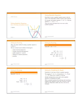
Statistical models come to rescue pe statistical models t benign l gn landscape s − − els tractable algorithms When data are generated by certain statistical / randomized models , problems are � �� � e.g. a k ∼ N ( 0 , I n ) often much nicer than worst-case instances

Convex relaxation Lifting: introduce X = xx ∗ to linearize constraints k x | 2 = a ∗ y k = | a ∗ k ( xx ∗ ) a k y k = a ∗ = ⇒ k Xa k

Convex relaxation Lifting: introduce X = xx ∗ to linearize constraints k x | 2 = a ∗ y k = | a ∗ k ( xx ∗ ) a k y k = a ∗ = ⇒ k Xa k X � 0 find y k = a ∗ k = 1 , · · · , m s.t. k Xa k , rank ( X ) = 1

Convex relaxation Lifting: introduce X = xx ∗ to linearize constraints k x | 2 = a ∗ y k = | a ∗ k ( xx ∗ ) a k y k = a ∗ = ⇒ k Xa k X � 0 find y k = a ∗ k = 1 , · · · , m s.t. k Xa k , rank ( X ) = 1

Convex relaxation Lifting: introduce X = xx ∗ to linearize constraints k x | 2 = a ∗ y k = | a ∗ k ( xx ∗ ) a k y k = a ∗ = ⇒ k Xa k X � 0 find y k = a ∗ k = 1 , · · · , m s.t. k Xa k , rank ( X ) = 1 Works well if { a k } are random

Convex relaxation Lifting: introduce X = xx ∗ to linearize constraints k x | 2 = a ∗ y k = | a ∗ k ( xx ∗ ) a k y k = a ∗ = ⇒ k Xa k X � 0 find y k = a ∗ k = 1 , · · · , m s.t. k Xa k , rank ( X ) = 1 Works well if { a k } are random, but huge increase in dimensions

Prior art (before our work) y = | Ax | 2 , A ∈ R m × n n : # unknowns; m : sample size (# eqns); sample complexity cvx relaxation n mn infeasible comput. cost

Prior art (before our work) y = | Ax | 2 , A ∈ R m × n n : # unknowns; m : sample size (# eqns); sample complexity infeasible cvx relaxation n mn infeasible comput. cost mn 2

Prior art (before our work) y = | Ax | 2 , A ∈ R m × n n : # unknowns; m : sample size (# eqns); sample complexity infeasible cvx relaxation n mn infeasible comput. cost mn 2 mn 2

Prior art (before our work) y = | Ax | 2 , A ∈ R m × n n : # unknowns; m : sample size (# eqns); sample complexity Wirtinger flow infeasible n log n 3 cvx relaxation n mn infeasible comput. cost mn 2 mn 2

Prior art (before our work) y = | Ax | 2 , A ∈ R m × n n : # unknowns; m : sample size (# eqns); sample complexity alt-min (fresh samples at each iter) n log 3 n Wirtinger flow infeasible n log n 3 cvx relaxation n mn infeasible comput. cost mn 2 mn 2

A glimpse of our results y = | Ax | 2 , A ∈ R m × n n : # unknowns; m : sample size (# eqns); sample complexity alt-min (fresh samples at each iter) n log 3 n Wirtinger flow infeasible n log n 3 cvx relaxation Our algorithm n mn infeasible comput. cost mn 2 mn 2 This work: random quadratic systems are solvable in linear time!

A glimpse of our results y = | Ax | 2 , A ∈ R m × n n : # unknowns; m : sample size (# eqns); sample complexity alt-min (fresh samples at each iter) n log 3 n Wirtinger flow infeasible n log n 3 cvx relaxation Our algorithm n mn infeasible comput. cost mn 2 mn 2 This work: random quadratic systems are solvable in linear time! � minimal sample size � optimal statistical accuracy

A first impulse: maximum likelihood estimate 1 � m minimize z f ( z ) = k =1 f k ( z ) m

A first impulse: maximum likelihood estimate 1 � m minimize z f ( z ) = k =1 f k ( z ) m k x | 2 + N (0 , σ 2 ) y k ∼ | a ∗ • Gaussian data: k z | 2 � 2 � y k − | a ∗ f k ( z ) =

A first impulse: maximum likelihood estimate 1 � m minimize z f ( z ) = k =1 f k ( z ) m k x | 2 + N (0 , σ 2 ) y k ∼ | a ∗ • Gaussian data: k z | 2 � 2 � y k − | a ∗ f k ( z ) = � k x | 2 � | a ∗ • Poisson data: y k ∼ Poisson k z | 2 − y k log | a ∗ f k ( z ) = | a ∗ k z | 2

A first impulse: maximum likelihood estimate 1 � m minimize z f ( z ) = k =1 f k ( z ) m k x | 2 + N (0 , σ 2 ) y k ∼ | a ∗ • Gaussian data: k z | 2 � 2 � y k − | a ∗ f k ( z ) = � k x | 2 � | a ∗ • Poisson data: y k ∼ Poisson k z | 2 − y k log | a ∗ f k ( z ) = | a ∗ k z | 2 Problem: f ( · ) nonconvex, many local stationary points

A plausible nonconvex paradigm � m minimize z f ( z ) = k =1 f k ( z ) ≈ h − i initial guess z 0 x basin of attraction 1. initialize within local basin sufficiently close to x � �� � (hopefully) nicer landscape

A plausible nonconvex paradigm � m minimize z f ( z ) = k =1 f k ( z ) ≈ h − i initial guess z 0 i ess z 0 z 1 z 2 x x basin of attraction basin of attraction 1. initialize within local basin sufficiently close to x � �� � (hopefully) nicer landscape 2. iterative refinement

Wirtinger flow (Cand` es, Li, Soltanolkotabi ’14) m f ( z ) = 1 � 2 − y k � �� � 2 a ⊤ minimize z k z m k =1 • spectral initialization: z 0 ← leading eigenvector of certain data matrix • (Wirtinger) gradient descent: z t +1 = z t − µ t ∇ f ( z t ) , t = 0 , 1 , · · ·

Performance guarantees for WF sample complexity alt-min (fresh samples at each iter) n log 3 n Wirtinger flow infeasible n log n 3 cvx relaxation Our algorithm n mn infeasible comput. cost mn 2 mn 2 • suboptimal computational cost? — n times more expensive than linear-time algorithms • suboptimal sample complexity?

Iterative refinement stage: search directions m z t +1 = z t − µ t � � k z t | 2 � y k − | a ⊤ a k a ⊤ k z t Wirtinger flow: m � �� � k =1 = ∇ f k ( z t )

Iterative refinement stage: search directions m z t +1 = z t − µ t � � k z t | 2 � y k − | a ⊤ a k a ⊤ k z t Wirtinger flow: m � �� � k =1 = ∇ f k ( z t ) Even in a local region around x (e.g. { z | � z − x � 2 ≤ 0 . 1 � x � 2 } ): • f ( · ) is NOT strongly convex unless m ≫ n • f ( · ) has huge smoothness parameter

Iterative refinement stage: search directions m z t +1 = z t − µ t � � k z t | 2 � y k − | a ⊤ a k a ⊤ k z t Wirtinger flow: m � �� � k =1 = ∇ f k ( z t ) x z locus of {∇ f k ( z ) } Problem: descent direction has large variability

Our solution: variance reduction via proper trimming More adaptive rule: m y i − | a ⊤ i z t | 2 z t +1 = z t − µ t � a i 1 E i 1 ( z t ) ∩E i 2 ( z t ) a ⊤ i z t m i =1 αh � � � y −A ( zz ⊤ ) 1 | a ⊤ � � � i z | � z ≤ | a ⊤ � � i z | where E i α lb � z � 2 ≤ α ub | y i − | a ⊤ i z | 2 | ≤ m ; E i � 1 ( z ) = 2 ( z ) = z � z � 2

Our solution: variance reduction via proper trimming More adaptive rule: m y i − | a ⊤ i z t | 2 z t +1 = z t − µ t � a i 1 E i 1 ( z t ) ∩E i 2 ( z t ) a ⊤ i z t m i =1 αh � � � y −A ( zz ⊤ ) 1 | a ⊤ � � � i z | � z ≤ | a ⊤ � � i z | where E i α lb � z � 2 ≤ α ub | y i − | a ⊤ i z | 2 | ≤ m ; E i � 1 ( z ) = 2 ( z ) = z � z � 2 x z

Our solution: variance reduction via proper trimming More adaptive rule: m y i − | a ⊤ i z t | 2 z t +1 = z t − µ t � a i 1 E i 1 ( z t ) ∩E i 2 ( z t ) a ⊤ i z t m i =1 αh � � � y −A ( zz ⊤ ) 1 | a ⊤ � � � i z | � z ≤ | a ⊤ � � i z | where E i α lb � z � 2 ≤ α ub | y i − | a ⊤ i z | 2 | ≤ m ; E i � 1 ( z ) = 2 ( z ) = z � z � 2 x informally, z t +1 = z t − µ z � k ∈T ∇ f k ( z t ) m • T trims away excessively large grad components