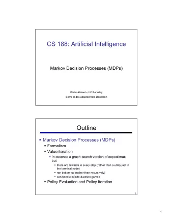
Solving Continuous MDPs with Discretization Pieter Abbeel UC - PowerPoint PPT Presentation
Solving Continuous MDPs with Discretization Pieter Abbeel UC Berkeley EECS Markov Decision Process Assumption: agent gets to observe the state [Drawing from Sutton and Barto, Reinforcement Learning: An Introduction, 1998] Markov Decision
Solving Continuous MDPs with Discretization Pieter Abbeel UC Berkeley EECS
Markov Decision Process Assumption: agent gets to observe the state [Drawing from Sutton and Barto, Reinforcement Learning: An Introduction, 1998]
Markov Decision Process (S, A, T, R, γ, H) Given S: set of states n A: set of actions n T: S x A x S x {0,1,…,H} à [0,1] T t (s,a,s’) = P(s t+1 = s’ | s t = s, a t =a) n R: S x A x S x {0, 1, …, H} à R t (s,a,s’) = reward for (s t+1 = s’, s t = s, a t =a) R n γ in (0,1]: discount factor H: horizon over which the agent will act n Goal: Find π *: S x {0, 1, …, H} à A that maximizes expected sum of rewards, i.e., n
Value Iteration Algorithm: Start with for all s. For i = 1, … , H For all states s in S: This is called a value update or Bellman update/back-up = expected sum of rewards accumulated starting from state s, acting optimally for i steps = optimal action when in state s and getting to act for i steps
Continuous State Spaces n S = continuous set n Value iteration becomes impractical as it requires to compute, for all states s in S:
Markov chain approximation to continuous state space dynamics model (“discretization”) n Original MDP n Discretized MDP ( ¯ S, ¯ A, ¯ T, ¯ R, γ , H ) (S, A, T, R, γ, H) Grid the state-space: the vertices are the discrete states. n Reduce the action space to a finite set. n n Sometimes not needed: n When Bellman back-up can be computed exactly over the continuous action space n When we know only certain controls are part of the optimal policy (e.g., when we know the problem has a “bang-bang” optimal solution) Transition function: see next few slides. n
Outline n Discretization n Lookahead policies n Examples n Guarantees n Connection with function approximation
Discretization Approach 1: Snap onto nearest vertex 0.1 a Discrete states: { ξ 1 , …, ξ 6 } 0.3 ξ 2 ξ 3 ξ 1 0.4 0.2 Similarly define transition probabilities for all ξ i ξ 4 ξ 5 ξ 6 Discrete MDP just over the states {ξ 1 , …,ξ 6 }, which we can solve with value iteration n If a (state, action) pair can results in infinitely many (or very many) different next states: n sample the next states from the next-state distribution
Discretization Approach 2: Stochastic Transition onto Neighboring Vertices ξ 1 ξ 2 ξ 3 ξ 4 Discrete states: {ξ 1 , …, ξ 12 } a s’ ξ 6 ξ 7 ξ 8 ξ 5 ξ 10 ξ 9 ξ 11 ξ 12 If stochastic dynamics: Repeat procedure to account for all possible transitions and weight accordingly n Many choices for p A , p B , p C , p D n
Discretization Approach 2: Stochastic Transition onto Neighboring Vertices One scheme to compute the weights: put in normalized coordinate system [0,1]x[0,1]. n ξ (1,1) ξ (1,0) 1 s’= (x,y) ξ (0,0) ξ (1,0) 0 1
Kuhn Triangulation** ξ 1 ξ 2 ξ 3 ξ 4 a s’ Discrete states: {ξ 1 , …, ξ 12 } ξ 6 ξ 7 ξ 8 ξ 5 ξ 10 ξ 9 ξ 11 ξ 12
Kuhn Triangulation** Allows efficient computation of the vertices participating in a point’s n barycentric coordinate system and of the convex interpolation weights (aka its barycentric coordinates) See Munos and Moore, 2001 for further details. n
Kuhn triangulation (from Munos and Moore)**
Discretization: Our Status n Have seen two ways to turn a continuous state-space MDP into a discrete state-space MDP n When we solve the discrete state-space MDP, we find: n Policy and value function for the discrete states n They are optimal for the discrete MDP, but typically not for the original MDP n Remaining questions: n How to act when in a state that is not in the discrete states set? n How close to optimal are the obtained policy and value function?
How to Act (i): No Lookahead For state s not in discretization set choose action based on policy in nearby states n Nearest Neighbor Stochastic Interpolation: n n Choose π ( ξ i ) with probability p i For continuous actions, can also interpolate: E.g., for s = p 2 ξ 2 + p 3 ξ 3 + p 6 ξ 6 , choose π ( ξ 2 ) , π ( ξ 3 ) , π ( ξ 6 ) with respective probabilities p 2 , p 3 , p 6
How to Act (ii): 1-step Lookahead Forward simulate for 1 step, calculate reward + value function at next state from discrete MDP n - if dynamics deterministic no expectation needed - If dynamics stochastic, can approximate with samples Stochastic Interpolation Nearest Neighbor n n
How to Act (iii): n-step Lookahead n What action space to maximize over, and how? n Option 1: Enumerate sequences of discrete actions we ran value iteration with n Option 2: Randomly sampled action sequences (“random shooting”) n Option 3: Run optimization over the actions n Local gradient descent [see later lectures] n Cross-entropy method
Intermezzo: Cross-Entropy Method (CEM) n CEM = black-box method for (approximately) solving: with and Note: f need not be differentiable
Intermezzo: Cross-Entropy Method (CEM) CEM: sample for iter i = 1, 2, … for e = 1, 2, … sample compute endfor
Intermezzo: Cross-Entropy Method (CEM) sigma and 10% are hyperparameters n can in principle also fit sigma to top 10% n (or full covariance matrix if low-D) How about discrete action spaces? n Within top 10%, look at frequency of each n discrete action in each time step, and use that as probability Then sample from this distribution n Note: there are many variations, including a max-ent variation, which does a weighted mean based on exp(f(x))
Outline n Discretization n Lookahead policies n Examples n Guarantees n Connection with function approximation
Mountain Car nearest neighbor #discrete values per state dimension: 20 #discrete actions: 2 (as in original env)
Mountain Car nearest neighbor #discrete values per state dimension: 150 #discrete actions: 2 (as in original env)
Mountain Car linear #discrete values per state dimension: 20 #discrete actions: 2 (as in original env)
Outline n Discretization n Lookahead policies n Examples n Guarantees n Connection with function approximation
Discretization Quality Guarantees n Typical guarantees: n Assume: smoothness of cost function, transition model n For h à 0, the discretized value function will approach the true value function n To obtain guarantee about resulting policy, combine above with a general result about MDP’s: n One-step lookahead policy based on value function V which is close to V* is a policy that attains value close to V*
Quality of Value Function Obtained from Discrete MDP: Proof Techniques n Chow and Tsitsiklis, 1991: Show that one discretized back-up is close to one “complete” back-up + then show sequence n of back-ups is also close n Kushner and Dupuis, 2001: Show that sample paths in discrete stochastic MDP approach sample paths in continuous n (deterministic) MDP [also proofs for stochastic continuous, bit more complex] n Function approximation based proof (see later slides for what is meant with “function approximation”) Great descriptions: Gordon, 1995; Tsitsiklis and Van Roy, 1996 n
Example result (Chow and Tsitsiklis,1991)**
Outline n Discretization n Lookahead policies n Examples n Guarantees n Connection with function approximation
Value Iteration with Function Approximation Alternative interpretation of the discretization methods: 0’th Order Function Approximation Start with for all s. For i = 0, 1, … , H-1 for all states , ( is the discrete state set) 1 st Order Function Approximation with:
Discretization as Function Approximation Nearest neighbor discretization: n builds piecewise constant approximation of value function - Stochastic transition onto nearest neighbors: n n-linear function approximation - Kuhn: piecewise (over “triangles”) linear approximation of value function -
Continuous time** One might want to discretize time in a variable way such that one discrete time transition roughly n corresponds to a transition into neighboring grid points/regions Discounting: n δt depends on the state and action See, e.g., Munos and Moore, 2001 for details. Note: Numerical methods research refers to this connection between time and space as the CFL (Courant Friedrichs Levy) condition. Googling for this term will give you more background info. !! 1 nearest neighbor tends to be especially sensitive to having the correct match [Indeed, with a mismatch between time and space 1 nearest neighbor might end up mapping many states to only transition to themselves no matter which action is taken.]
Recommend
More recommend
Explore More Topics
Stay informed with curated content and fresh updates.
