Slits, spirals and Loewner hulls Joan Lind University of Tennessee - PowerPoint PPT Presentation

Slits, spirals and Loewner hulls Joan Lind University of Tennessee

The story begins Bieberbach conjecture (1916): For f ( z ) = z + a 2 z 2 + a 3 z 3 + · · · conformal on D , then | a n | ≤ n .

The story begins Bieberbach conjecture (1916): For f ( z ) = z + a 2 z 2 + a 3 z 3 + · · · conformal on D , then | a n | ≤ n . Charles Loewner introduced the Loewner equation in 1923 to prove the n = 3 case.

The story begins Bieberbach conjecture (1916): For f ( z ) = z + a 2 z 2 + a 3 z 3 + · · · conformal on D , then | a n | ≤ n . Charles Loewner introduced the Loewner equation in 1923 to prove the n = 3 case. Louis des Branges again used the Loewner equation when he proved the conjecture in 1985.

The story continues 0 Simple Random Walk (SRW) in 2 dimensions – has a conformally invariant scaling limit: 2-d Brownian motion

The story continues Schramm’s question: Do other 2-dimensional random walks (such as SAW, LERW, etc.) have conformally invariant scaling limits? 0

The story continues In 2000, Oded Schramm introduced SLE κ , a family of random processes that contain the possible conformally invariant scaling limits.

The story continues In 2000, Oded Schramm introduced SLE κ , a family of random processes that contain the possible conformally invariant scaling limits. Through the Loewner equation, SLE κ correspond to √ κ B t .

The Loewner equation L Equ ← ! growing families of 2-d sets real-valued functions

From curves to functions γ ( t )

From curves to functions γ ( t )

From curves to functions g t γ ( t ) λ ( t )

From curves to functions g t γ ( t ) λ ( t ) � 1 g t ( z ) = z + c t � z + O for z near infinity z 2

From curves to functions g t γ ( t ) λ ( t ) � 1 g t ( z ) = z + 2 t � z + O for z near infinity z 2

From curves to functions g t γ ( t ) λ ( t ) ∂ 2 ∂ t g t ( z ) = g t ( z ) − λ ( t )

From functions to growing families of sets For a continuous, real-valued function λ ( t ) and z ∈ H , consider ∂ 2 ∂ t g t ( z ) = g t ( z ) − λ ( t ) , g 0 ( z ) = z

From functions to growing families of sets For a continuous, real-valued function λ ( t ) and z ∈ H , consider ∂ 2 ∂ t g t ( z ) = g t ( z ) − λ ( t ) , g 0 ( z ) = z Loewner hulls: K t = { z ∈ H : g s ( z ) = λ ( s ) for some s ≤ t } .

From functions to growing families of sets For a continuous, real-valued function λ ( t ) and z ∈ H , consider ∂ 2 ∂ t g t ( z ) = g t ( z ) − λ ( t ) , g 0 ( z ) = z Loewner hulls: K t = { z ∈ H : g s ( z ) = λ ( s ) for some s ≤ t } . Theorem: g t is a conformal map from H \ K t onto H .

Loewner flow ∂ t g t ( z ) = 2 Re g t ( z ) − λ ( t ) ∂ Im g t ( z ) | g t ( z ) − λ ( t ) | 2 − 2 i | g t ( z ) − λ ( t ) | 2 1 0.8 0.6 0.4 0.2 –1 –0.5 0.5 1

Example Loewner hull generated by λ ( t ) ≡ 0.

Loewner equation L Equ ← ! growing families of 2-d sets real-valued functions

The geometry of SLE curves L Equ √ κ B t SLE κ ← →

The geometry of SLE curves L Equ √ κ B t SLE κ ← → 0 ≤ κ ≤ 4 4 < κ < 8 8 ≤ κ

The geometry of SLE curves SLE 2 SLE 6

Simple curve Loewner hulls Question: When does the deterministic Loewner equation generate a simple curve?

Simple curve Loewner hulls Question: When does the deterministic Loewner equation generate a simple curve? Lip(1 / 2) functions: | λ ( t ) − λ ( s ) | ≤ M | t − s | 1 / 2 for all t , s is the domain of λ. The smallest such M is || λ || 1 / 2 .

Simple curve Loewner hulls Question: When does the deterministic Loewner equation generate a simple curve? Lip(1 / 2) functions: | λ ( t ) − λ ( s ) | ≤ M | t − s | 1 / 2 for all t , s is the domain of λ. The smallest such M is || λ || 1 / 2 . Answer: (Marshall, Rohde) There exists C 0 > 0 so that for λ ∈ Lip(1 / 2) with || λ || 1 / 2 < C 0 , then the Loewner hull is a quasislit γ .

Simple curve Loewner hulls Question: Do all Lip(1 / 2) driving functions generate simple curves?

Simple curve Loewner hulls Question: Do all Lip(1 / 2) driving functions generate simple curves? Answer: (Marshall, Rohde) No. There is a non-simple example (a curve that spirals around a disc) that is generated by a Lip(1 / 2) driving function.

Simple curve Loewner hulls Question: What is the optimal value of C 0 for the Marshall-Rohde theorem?

Simple curve Loewner hulls Question: What is the optimal value of C 0 for the Marshall-Rohde theorem? Answer: (L) C 0 = 4.

Simple curve Loewner hulls Question: What is the optimal value of C 0 for the Marshall-Rohde theorem? Answer: (L) C 0 = 4. Key examples: λ ( t ) = − c √ 1 − t c = 3 c = 5

Loewner deformations Omer Angel’s question: For r < 1, what can you say about Loewner hull driven by r λ ?

Loewner deformations Omer Angel’s question: For r < 1, what can you say about Loewner hull driven by r λ ? Is it at least as nice as the hull driven by λ ?

Loewner deformations Omer Angel’s question: For r < 1, what can you say about Loewner hull driven by r λ ? Is it at least as nice as the hull driven by λ ? This is true for SLE. 0 ≤ κ ≤ 4 4 < κ < 8 8 ≤ κ

Loewner deformations Omer Angel’s question: For r < 1, what can you say about Loewner hull driven by r λ ? Is it at least as nice as the hull driven by λ ? This is true for λ ( t ) = − c √ 1 − t . c = 3 c = 5

Loewner deformations Omer Angel’s question: For r < 1, what can you say about Loewner hull driven by r λ ? Is it at least as nice as the hull driven by λ ? Is it always true?

Loewner deformations Omer Angel’s question: For r < 1, what can you say about Loewner hull driven by r λ ? Is it at least as nice as the hull driven by λ ? Is it always true? Answer: N0.

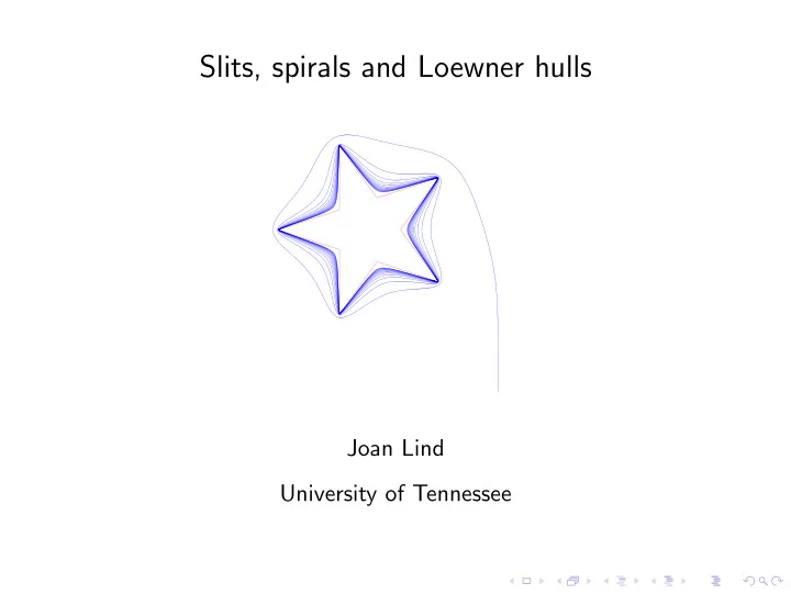
Loewner deformations Theorem (L, Marshall, Rohde) Let λ be the driving function for the star spiral. When 0 < r < 1 , then r λ generates a simple curve, and when r > 1 , then r λ generates a “bubble” curve.

Spirals and collisions Theorem (L, Marshall, Rohde) If γ is a suffiently nice infinite spiral of half-plane capacity T, or if γ has a tangential self-intersection, then its driving term λ satisfies | λ ( T ) − λ ( t ) | lim √ = 4 . T − t t → T

Spirals and collisions Theorem (L, Marshall, Rohde) If γ is a suffiently nice infinite spiral of half-plane capacity T, or if γ has a tangential self-intersection, then its driving term λ satisfies | λ ( T ) − λ ( t ) | lim √ = 4 . T − t t → T Theorem (L, Marshall, Rohde) If λ : [0 , T ] → R is sufficiently regular on [0 , T ) and if | λ ( T ) − λ ( t ) | √ lim = κ > 4 , T − t t → T then γ ( T ) = lim t → T γ ( t ) exists, is real, and γ intersects R in the same angle as the trace for κ √ 1 − t.

Spirals and collisions Scaling Property: ◮ If λ generates hull K t , then c λ ( t / c 2 ) generates cK t / c 2 .

Spirals and collisions Scaling Property: ◮ If λ generates hull K t , then c λ ( t / c 2 ) generates cK t / c 2 . Example: λ ( t ) = c √ t

Spirals and collisions Concatenation Property: ◮ If λ generates hull K t for t ∈ [0 , T ], then λ restricted to [ t 0 , T ] generates hull g t 0 ( K T \ K t 0 ).

Spirals and collisions Concatenation Property: ◮ If λ generates hull K t for t ∈ [0 , T ], then λ restricted to [ t 0 , T ] generates hull g t 0 ( K T \ K t 0 ). g t 0 g t 0 ( K T \ K t 0 ) K t 0 λ (0) λ ( t 0 )

Spirals and collisions Start with λ = − c √ 1 − t . For t 0 ∈ (0 , 1), map down by g t 0 . Rescale by 1 / √ 1 − t 0 .

Spirals and collisions Start with λ = − c √ 1 − t . For t 0 ∈ (0 , 1), map down by g t 0 . Rescale by 1 / √ 1 − t 0 . What do we obtain? The same hull that we started with.

Spirals and collisions Start with λ satisfying | λ (1) − λ ( t ) | lim √ 1 − t = κ ≥ 4 t → 1 Shift so that λ (1) = 0. For t 0 ∈ (0 , 1), map down by g t 0 . Rescale by 1 / √ 1 − t 0 .

Spirals and collisions Start with λ satisfying | λ (1) − λ ( t ) | lim √ 1 − t = κ ≥ 4 t → 1 Shift so that λ (1) = 0. For t 0 ∈ (0 , 1), map down by g t 0 . Rescale by 1 / √ 1 − t 0 . What do we obtain? A hull that is getting closer and closer to the hull generated by ± κ √ 1 − t .

Spirals and collisions What happens when κ = 4?

Spirals and collisions What happens when κ = 4? 4 √ 1 − t generates a hull that intersects the real line tangentially.

Spirals and collisions What happens when κ = 4? 4 √ 1 − t generates a hull that intersects the real line tangentially. The spiral behavior can be viewed as tangential behavior.

Recap: the Loewner equation question L Equ ← ! growing families of 2-d sets real-valued functions Question: How do properties of the functions relate to geometric characteristics of the sets?

Sample of other Loewner explorations

Sample of other Loewner explorations ◮ Spacefilling curves (L, Rohde)

Sample of other Loewner explorations ◮ Spacefilling curves (L, Rohde) ◮ Driving functions with higher regularity (Wong, L, Tran)