COMS 4721: Machine Learning for Data Science Lecture 11, 2/23/2017 - PowerPoint PPT Presentation
COMS 4721: Machine Learning for Data Science Lecture 11, 2/23/2017 Prof. John Paisley Department of Electrical Engineering & Data Science Institute Columbia University M AXIMUM M ARGIN C LASSIFIERS M AXIMUM MARGIN IDEA Setting Linear
COMS 4721: Machine Learning for Data Science Lecture 11, 2/23/2017 Prof. John Paisley Department of Electrical Engineering & Data Science Institute Columbia University
M AXIMUM M ARGIN C LASSIFIERS
M AXIMUM MARGIN IDEA Setting Linear classification, two linearly separable classes. Recall Perceptron ◮ Selects some hyperplane separating the classes. ◮ Selected hyperplane depends on several factors. Maximum margin To achieve good generalization (low prediction error), place the hyperplane “in the middle” between the two classes. More precisely, choose a plane such that its distance to the closest point in each class is maximized. This distance is called the margin .
G ENERALIZATION E RROR Possible Perceptron solution (dotted) poor generalization, (solid) better Maximum margin solution Example: Gaussian data ◮ Intuitively, the classifier on the left isn’t good because sampling more data could lead to misclassifications. ◮ If we imagine the data from each class as Gaussian, we could frame the goal as to find a decision boundary that cuts into as little probability mass as possible. ◮ With no distribution assumptions, we can argue that max-margin is best.
S UBSTITUTING CONVEX SETS Observation Where a separating hyperplane may be placed depends on the “outer” points on the sets. Points in the center do not matter. In geometric terms, we can represent each class by the smallest convex set which contains all point in the class. This is called a convex hull .
S UBSTITUTING CONVEX SETS Convex hulls The thing to remember for this lecture is that a convex hull is defined by all possible weighted averages of points in a set. That is, let x 1 , . . . , x n be the above data coordinates. Every point x 0 in the shaded region – i.e., the convex hull – can be reached by setting n n � � x 0 = α i x i , α i ≥ 0 , α i = 1 , i = 1 i = 1 for some ( α 1 , . . . , α n ) . No point outside this region can be reached this way.
M ARGIN Definition The margin of a classifying hyperplane H is the shortest distance between the plane and any point in either set (equivalently, the convex hull) When we maximize this margin, H is “exactly in the middle” of the two convex hulls. Of course, the difficult part is how do we find this H ?
S UPPORT VECTOR MACHINES
S UPPORT V ECTOR M ACHINE Finding the hyperplane For n linearly separable points ( x 1 , y 1 ) , . . . , ( x n , y n ) with y i ∈ {± 1 } , solve: 1 2 � w � 2 min w , w 0 y i ( x T i w + w 0 ) ≥ 1 for i = 1 , . . . , n subject to Comments ◮ Recall that y i ( x T i w + w 0 ) > 0 if y i = sign ( x T i w + w 0 ) . ◮ If there exists a hyperplane H that separates the classes, we can scale w so that y i ( x T i w + w 0 ) > 1 for all i (this is useful later). ◮ The resulting classifier is called a support vector machine . This formulation only has a solution when the classes are linearly separable. ◮ It is not at all obvious why this maximizes the margin. This will become more clear when we look at the solution.
S UPPORT V ECTOR M ACHINE Skip to the end Q : First, can we intuitively say what the solution should look like? A : Yes, but we won’t give the proof. 1 . Find the closest two points from the convex hulls of class + 1 and − 1. 2 . Connect them with a line and put a perpendicular hyperplane in the middle. 3 . If S 1 and S 0 are the sets of x in class + 1 and − 1 respectively, we’re looking for two probability vectors α 1 and α 0 such that we minimize � � � ( � − ( � � � x i ∈ S 1 α 1 i x i ) x i ∈ S 0 α 0 i x i ) � 2 � �� � � �� � in conv. hull of S 1 in conv. hull of S 0 4 . Then we define the hyperplane using the two points found with α 1 and α 0 .
P RIMAL AND D UAL PROBLEMS Primal problem The primal optimization problem is the one we defined: 1 2 � w � 2 min w , w 0 y i ( x T i w + w 0 ) ≥ 1 for i = 1 , . . . , n subject to This is tricky, so we use Lagrange multipliers to set up the “dual” problem. Lagrange multipliers Define Lagrange multipliers α i > 0 for i = 1 , . . . , n . The Lagrangian is n 1 � 2 � w � 2 − α i ( y i ( x T L = i w + w 0 ) − 1 ) i = 1 n n 1 � � 2 � w � 2 − α i y i ( x T = i w + w 0 ) + α i i = 1 i = 1 We want to minimize L over w and w 0 and maximize over ( α 1 , . . . , α n ) .
S ETTING UP THE DUAL PROBLEM First minimize over w and w 0 : n n L = 1 � � 2 � w � 2 − α i y i ( x T i w + w 0 ) + α i i = 1 i = 1 ⇓ n n � � ∇ w L = w − α i y i x i = 0 ⇒ w = α i y i x i i = 1 i = 1 n n ∂ L � � = − α i y i = 0 ⇒ α i y i = 0 ∂ w 0 i = 1 i = 1 Therefore, 1. We can plug the solution for w back into the problem. 2. We know that ( α 1 , . . . , α n ) must satisfy � n i = 1 α i y i = 0.
SVM DUAL PROBLEM 2 � w � 2 − � n i w + w 0 ) + � n Lagrangian : L = 1 i = 1 α i y i ( x T i = 1 α i Dual problem Plugging these values in from the previous slide, we get the dual problem n n n α i − 1 � � � α i α j y i y j ( x T max L = i x j ) 2 α 1 ,...,α n i = 1 i = 1 j = 1 n � α i y i = 0 , α i ≥ 0 for i = 1 , . . . , n subject to i = 1 Comments ◮ Where did w 0 go? The condition � n i = 1 α i y i = 0 gives 0 · w 0 in the dual. ◮ We now maximize over the α i . This requires an algorithm that we won’t discuss in class. Many good software implementations are available.
A FTER SOLVING THE DUAL Solving the primal problem Before discussing the solution of the dual, we ask: After finding each α i how do we predict a new y 0 = sign ( x T 0 w + w 0 ) ? 2 � w � 2 − � n L = 1 i = 1 α i ( y i ( x T We have: i w + w 0 ) − 1 ) α i ≥ 0 , y i ( x T i w + w 0 ) − 1 ≥ 0 With conditions: Solve for w . n � ∇ w L = 0 ⇒ w = α i y i x i (just plug in the learned α i ’s) i = 1 What about w 0 ? ◮ We can show that at the solution, α i ( y i ( x T i w + w 0 ) − 1 ) = 0 for all i . ◮ Therefore, pick i for which α i > 0 and solve y i ( x T i w + w 0 ) − 1 = 0 for w 0 using the solution for w (all possible i will give the same solution).
U NDERSTANDING THE DUAL Dual problem We can manipulate the dual problem to find out what it’s trying to do. n n n α i − 1 � � � α i α j y i y j ( x T L = i x j ) max 2 α 1 ,...,α n i = 1 i = 1 j = 1 n � α i y i = 0 , α i ≥ 0 for i = 1 , . . . , n subject to i = 1 Since y i ∈ {− 1 , + 1 } n � � � α i y i = 0 ⇒ C = α i = α j ◮ i = 1 i ∈ S 1 j ∈ S 0 n n n � � = C 2 � � 2 α i α j 2 � � � � � α i α j y i y j ( x T � � � � i x j ) = α i y i x i C x i − C x j ◮ � � � � i = 1 j = 1 i = 1 i ∈ S 1 j ∈ S 0
U NDERSTANDING THE DUAL Dual problem We can change notation to write the dual as 2 C 2 � � L = 2 C − 1 α i α j 2 � � � � C x i − max C x j � � α 1 ,...,α n i ∈ S 1 j ∈ S 0 � � C := α i = α j , α i ≥ 0 subject to i ∈ S 1 j ∈ S 0 We observe that the maximum of this function satisfies � � � � � �� � 2 α j � α i � min C x i − C x j � � i ∈ S 1 j ∈ S 0 α 1 ,...,α n � �� � � �� � in conv. hull of S 1 in conv. hull of S 0 Therefore, the dual problem is trying to find the closest points in the convex hulls constructed from data in class + 1 and − 1.
R ETURNING TO THE PICTURE Recall We wanted to find: � u − v � 2 min u ∈H ( S 1 ) v ∈H ( S 0 ) The direction of w is u − v . We previously claimed we can find the max-margin hyperplane as follows: 1. Find shortest line connecting the convex hulls. 2. Place hyperplane orthogonal to line and exactly at the midpoint. With the SVM we want to minimize � w � 2 and we can write this solution as n α i α j � � � w = α i y i x i = C C x i − C x j i = 1 i ∈ S 1 j ∈ S 0
S OFT - MARGIN SVM Question : What if the data isn’t linearly separable? Answer : Permit training data be on wrong side of hyperplane, but at a cost. Slack variables Replace the training rule y i ( x T i w + w 0 ) ≥ 1 with y i ( x T i w + w 0 ) ≥ 1 − ξ i , with ξ i ≥ 0. ξ > 1 The ξ i are called slack variables . ξ < 1 ξ = 0 ξ = 0
S OFT -M ARGIN SVM Soft-margin objective function Adding the slack variables gives a new objective to optimize n 1 � 2 � w � 2 + λ ξ i min w , w 0 ,ξ 1 ,...,ξ n i = 1 y i ( x T subject to i w + w 0 ) ≥ 1 − ξ i for i = 1 , . . . , n ξ i ≥ 0 for i = 1 , . . . , n We also have to choose the parameter λ > 0. We solve the dual as before. Role of λ ◮ Specifies the “cost” of allowing a point on the wrong side. ◮ If λ is very small, we’re happy to misclassify. ◮ For λ → ∞ , we recover the original SVM because we want ξ i = 0. ◮ We can use cross-validation to choose it.
I NFLUENCE OF M ARGIN P ARAMETER λ = 100000 λ = 0 . 01 Hyperplane is sensitive to λ . Either way, a linear classifier isn’t ideal . . .
Recommend
More recommend
Explore More Topics
Stay informed with curated content and fresh updates.
