Slide Set 3 Notes Regression Models and the Classical Linear - PowerPoint PPT Presentation
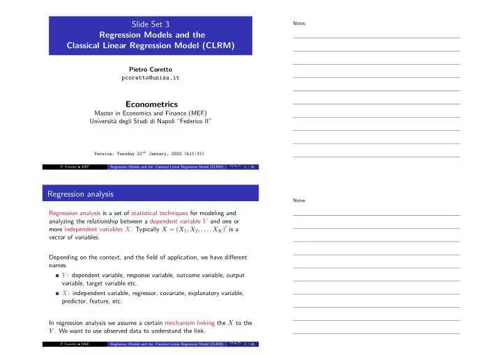
Slide Set 3 Notes Regression Models and the Classical Linear Regression Model (CLRM) Pietro Coretto pcoretto@unisa.it Econometrics Master in Economics and Finance (MEF) Universit degli Studi di Napoli Federico II Version: Tuesday 21
Slide Set 3 Notes Regression Models and the Classical Linear Regression Model (CLRM) Pietro Coretto pcoretto@unisa.it Econometrics Master in Economics and Finance (MEF) Università degli Studi di Napoli “Federico II” Version: Tuesday 21 st January, 2020 (h11:31) P. Coretto • MEF Regression Models and the Classical Linear Regression Model (CLRM) 1 / 26 Regression analysis Notes Regression analysis is a set of statistical techniques for modeling and analyzing the relationship between a dependent variable Y and one or more independent variables X . Typically X = ( X 1 , X 2 , . . . , X K ) ′ is a vector of variables. Depending on the context, and the field of application, we have different names Y : dependent variable, response variable, outcome variable, output variable, target variable etc. X : independent variable, regressor, covariate, explanatory variable, predictor, feature, etc. In regression analysis we assume a certain mechanism linking the X to the Y . We want to use observed data to understand the link. P. Coretto • MEF Regression Models and the Classical Linear Regression Model (CLRM) 2 / 26
Regression function and types of regression models Notes The link is formalized in terms of a regression function. The latter models the relationship between Y and X Y ≈ f ( X ) Building a regression model requires to specify how the f ( · ) transforms X in which sense the f ( · ) approximates Y P. Coretto • MEF Regression Models and the Classical Linear Regression Model (CLRM) 3 / 26 Notes Depending on how the f ( · ) transforms X we have nonparametric models parametric models Nonparametric models The f ( · ) is treated as the unknown. Therefore the object of interest belongs to an infinite dimensional space. Usually we restrict our quest to some well defined class, for instance we may restrict the analysis to � � � f : f is real valued, smooth and | f ( x ) | dx < + ∞ Nonparametric models allow for a lot flexibility, and this comes at a price. P. Coretto • MEF Regression Models and the Classical Linear Regression Model (CLRM) 4 / 26
Parametric models f is assumed to have a specific form controlled by a scalar parameter β or Notes a vector of parameters β = ( β 1 , β 2 , . . . , β p ) ′ . Therefore the object of interest is β . Examples linear parametric regession function: f ( X ; β ) = β 1 X 1 + β 2 X 2 nonlinear parametric regession function: f ( X ; β ) = sin( β 1 X 1 ) + e β 2 X 2 Some nonlinear regression function can be linearized. Example: f ( X ; β ) = e X 1 + βX 2 − → log( f ( X ; β )) = X 1 + βX 2 Sometimes a regression function is not linear in the original X , but it is linear in a transformation of X f ( X ; β ) = β 1 X 2 1 + β 2 X 2 P. Coretto • MEF Regression Models and the Classical Linear Regression Model (CLRM) 5 / 26 Notes Depending on what kind of approximation f ( · ) provides about Y (conditional) mean regression: f ( X ) = E[ Y | X ] (conditional) quantile regression: f ( X ) = median [ Y | X ] f ( X ) = quantile α [ Y | X ] etc... Conditional mean regression functions are central in regression analysis for several reasons: approximating Y by an average it’s intuitive most theoretical models are expressed in terms of expectations “ Optimal Predictor Theorem ” P. Coretto • MEF Regression Models and the Classical Linear Regression Model (CLRM) 6 / 26
The quality of the approximation Y ≈ f ( X ) can be measure by the Notes quadratic risk or MSE E[( Y − f ( X )) 2 ] Theorem (Optimal Predictor) Under suitable regularity conditions E[( Y − f ( X )) 2 ] = E[ Y | X ] inf f In other words f ( X ) = E[ Y | X ] gives the best approximation to Y in terms of MSE If we want to guess Y based on information generated by X , f ( X ) = E[ Y | X ] is the best guess in terms of MSE P. Coretto • MEF Regression Models and the Classical Linear Regression Model (CLRM) 7 / 26 Proof. We need to show that for any function f ( X ) Notes E[( Y − E[ Y | X ]) 2 ] ≤ E[( Y − f ( X )) 2 ] 2 E[( Y − f ( X )) 2 ] = E Y − E[ Y | X ] + E[ Y | X ] − f ( X ) � �� � � �� � A B computing ( A + B ) 2 and using using the lineary of expectations E[ A 2 ] + E[ B 2 ] + 2 E[ AB ] = E[( Y − f ( X )) 2 ] (3.1) E[ B 2 ] = E[(E[ Y | X ] − f ( X )) 2 ] ≥ 0 , therefore (3.1) becomes E[ A 2 ] + 2 E[ AB ] ≤ E[( Y − f ( X )) 2 ] (3.2) P. Coretto • MEF Regression Models and the Classical Linear Regression Model (CLRM) 8 / 26
Notes E[ AB ] = E[ E[ AB | X ] ] (law of iterated expectations ) � ( Y − E[ Y | X ])(E[ Y | X ] − f ( X )) � � � X = E � ( Y − E[ Y | X ]) � � � X = (E[ Y | X ] − f ( X )) E (pull out) = (E[ Y | X ] − f ( X )) { E[ Y | X ] − E[E[ Y | X ] | X ] } = (E[ Y | X ] − f ( X )) × 0 Therefore, (3.2) becomes E[ A 2 ] ≤ E[( Y − f ( X )) 2 ] with E[ A 2 ] = E[( Y − E[ Y | X ]) 2 ] , which proves the result � P. Coretto • MEF Regression Models and the Classical Linear Regression Model (CLRM) 9 / 26 Notes In this course we focus on conditional mean regression models where the regression function has a linear parametric form: Y ≈ E[ Y | X ] = f ( X ; β ) = β 1 X 1 + β 2 X 2 + . . . + β K X K The reason why this class of regression models is so popular is that because they can reproduce correlation between Y and X s. Going back to the example of Slide Set #1 P. Coretto • MEF Regression Models and the Classical Linear Regression Model (CLRM) 10 / 26
Notes 250 200 Y 150 100 50 5 10 15 20 X P. Coretto • MEF Regression Models and the Classical Linear Regression Model (CLRM) 11 / 26 Notes Y y | x = 135 . 1 ¯ x = 5 X P. Coretto • MEF Regression Models and the Classical Linear Regression Model (CLRM) 12 / 26
Notes y | x = 171 . 8 Y ¯ x = 10 X P. Coretto • MEF Regression Models and the Classical Linear Regression Model (CLRM) 13 / 26 Notes y | x = 208 . 6 ¯ Y x = 15 X P. Coretto • MEF Regression Models and the Classical Linear Regression Model (CLRM) 14 / 26
The model postulates that Y ≈ E[ Y | X ] , but we cannot observe E[ Y | X ] . Notes For each sample unit i = 1 , 2 , . . . , n we observe the samples ( Y i , X i 1 , X i 2 , . . . , X ik ) . Therefore, we need an additional term which summarizes the difference between Y i and its conditional mean E[ Y i | X ] A way to reproduce the previous sampling mechanism is to add an error term ε i , which is a random variable that “ summarizes ” the deviations of Y i from its conditional mean E[ Y i | X ] . Therefore Y i = f ( X i ; β ) + ε i = E[ Y i | X ] + ε i = β 1 X 1 + β 2 X 2 + . . . + β K X K + ε i The short name for this class of models is linear regression models = linear parametric regression function plus an additive error term. P. Coretto • MEF Regression Models and the Classical Linear Regression Model (CLRM) 15 / 26 Partial or marginal effects Notes The partial/marginal effect is a measure of the effect on the regression function determined by a change in a regressor X j holding all the other regressors constant (waee = “ with all else equal ”). Let us focus on conditional mean models. Assuming differentiability, the partial/marginal effect of a change ∆ X j is given by ∆ E[ Y | X ] = ∂ E[ Y | X ] ∆ X j hoding fixed X 1 , . . . , X j − 1 , X j +1 , . . . , X K ∂X j Computing marginal/partial effects make sense only when the model has a causal interpretation (see later). P. Coretto • MEF Regression Models and the Classical Linear Regression Model (CLRM) 16 / 26
For the linear regression model Notes ∂ E[ Y | X ] = β j ∂X j Therefore, the unknown parameters β j coincides with partial effect of an unit change in X j waee . For a discrete regressor X j , partial effects are computed as the variations in E[ Y | X ] obtained by changing the level of X j and waee . Suppose X k ∈ { a, b, c } . The partial effect when X k changes from level a to b ( waee ) is given by E[ Y | X k = b, X ] − E[ Y | X k = a, X ] Another measure of regressors’ effect on the Y is the partial/marginal elasticity (see homeworks). P. Coretto • MEF Regression Models and the Classical Linear Regression Model (CLRM) 17 / 26 Notations Notes Indexes and constants: n : number of sample units K : number of covariates/regressors/features measured on each of the n sample units i = 1 , 2 , . . . , n : indexes sample units k = 1 , 2 , . . . , K : indexes regressors y ∈ R n : column vector of the dependent/response variable y 1 y 2 y = . . . y n P. Coretto • MEF Regression Models and the Classical Linear Regression Model (CLRM) 18 / 26
x i ∈ R K : column vector containing the K regressors measured on the Notes i th sample unit x i 1 x i 2 x i = . . . x iK So called design matrix, is the ( n × K ) matrix whose rows contain sample units and columns contain regressors x 11 x 12 . . . x 1 K x 1 ′ x 2 ′ x 21 x 22 . . . x 2 K X = = . . ... . . . . . . . . . . x n ′ x n 1 x n 2 . . . x nK P. Coretto • MEF Regression Models and the Classical Linear Regression Model (CLRM) 19 / 26 Notes ε ∈ R n : column vector containing the error term for each unit ε 1 ε 2 ε = . . . ε n P. Coretto • MEF Regression Models and the Classical Linear Regression Model (CLRM) 20 / 26
Recommend
More recommend
Explore More Topics
Stay informed with curated content and fresh updates.
