Simplified analysis of phase transitions in thermodynamics Jay Wang - PDF document

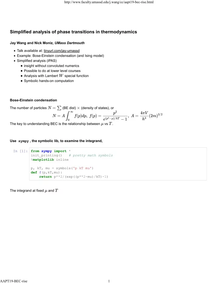
http://www.faculty.umassd.edu/j.wang/cc/aapt19-bec-rise.html Simplified analysis of phase transitions in thermodynamics Jay Wang and Nick Moniz, UMass Dartmouth Talk available at: tinyurl.com/jay-umassd Example: Bose-Einstein condensation (and Ising model) Simplified analysis (iPAS) insight without convoluted numerics Possible to do at lower level courses Analysis with Lambert special function Symbolic hands-on computation Bose-Einstein condensation The number of particles (BE dist) (density of states), or The key to understanding BEC is the relationship between vs . Use sympy , the symbolic lib, to examine the integrand, In [1]: from sympy import * init_printing() # pretty math symbols % matplotlib inline p, kT, mu = symbols('p kT mu') def f(p,kT,mu): return p**2/(exp((p**2-mu)/kT)-1) The integrand at fixed and AAPT19-BEC-rise 1

http://www.faculty.umassd.edu/j.wang/cc/aapt19-bec-rise.html In [2]: plt = plot(f(p,kT=2,mu=-1), f(p,kT=1,mu=-1), ### Fixed chem. pot. xlim=[0,3], legend=1, show=0) plt[0].label='$kT=2$'; plt[1].line_color='red'; plt[1].label='$kT=1$' plt.show() In [3]: plt = plot(f(p,kT=1,mu=-.5), f(p,kT=1,mu=-1), ### Fixed T xlim=[0,3], legend=1, show=0) plt[0].label='$\mu=-0.5$'; plt[1].line_color='red'; plt[1].label='$\mu=-1$' plt.show() So, must increase when decreases to conserve particle number . Quantitatively, one must either do some numerical acrobatics; or some simplification . We choose the latter, semiquantitatively correct and suitable for lower level courses. Assumption : The area is proportional to the height of the peak, AAPT19-BEC-rise 2

http://www.faculty.umassd.edu/j.wang/cc/aapt19-bec-rise.html This is justified because the width varies much slower than height (details in Am. J. Phys. 2019, accepted) Effectively, , some scaled particle number. To find the maximum, set , In [4]: dfdp = diff(f(p,kT,mu), p) # derivative, f'(p) dfdp Out[4]: Solve for , In [5]: pmax = solve(dfdp, p) # find maximum pmax Out[5]: Note the Lambert function appears (more on it later). To find and find , In [6]: fmax=f(pmax[1],kT,mu) fmax Out[6]: which simplifies to ( sympy needs a bit help at times) In [7]: fmax = -kT*LambertW(-exp(mu/kT-1)) fmax Out[7]: AAPT19-BEC-rise 3

http://www.faculty.umassd.edu/j.wang/cc/aapt19-bec-rise.html Recall represents the area (or ) Now as decreases, must adjust such that , say (equiv ) for some fixed . Solve for In [8]: u = solve(fmax-1, mu) u Out[8]: or make it tidier, Central closed-form result : how changes to keep constant. Relationship between and , critical temperature at In [9]: plot(u[0], (kT,1,3), xlim=[0,3], ylim=[-1,.1]); The maximum of is zero. What if continues to decrease? Because after , it can no longer compensate for the shrinking integral. Evidently, the "missing" particles fall into the ground state, the Bose-Einstein condensate, i.e., AAPT19-BEC-rise 4

http://www.faculty.umassd.edu/j.wang/cc/aapt19-bec-rise.html 1- The Lambert function: defined as the satisfying In [10]: x = symbols('x') W = LambertW # shorthand plt = plot(W(x,0), W(x,-1), xlim=[-.5,4], ylim=[-5,2], legend=1, show=0) plt[0].label='$W_0$'; plt[1].line_color='red'; plt[1].label='$W_{-1}$'; plt.show() In [11]: diff(W(x),x) Out[11]: In [12]: integrate(W(x),x) Out[12]: Discussion Simplified analysis of BEC with the function; Ising model may be solved similarly (AJP 2019 accepted) The function recently used in CM, QM, thermo, chaos, helio- & astro-phys, eco-bio systems, supply-chain problems Potential application to yet unknown thermal problems due to FD and BE distributions involving Talk available at: tinyurl.com/jay-umassd AAPT19-BEC-rise 5