SHANNONS INFORMATION THEORY ITS APPLICATIONS IN DERIVATIVE PRICING - PDF document

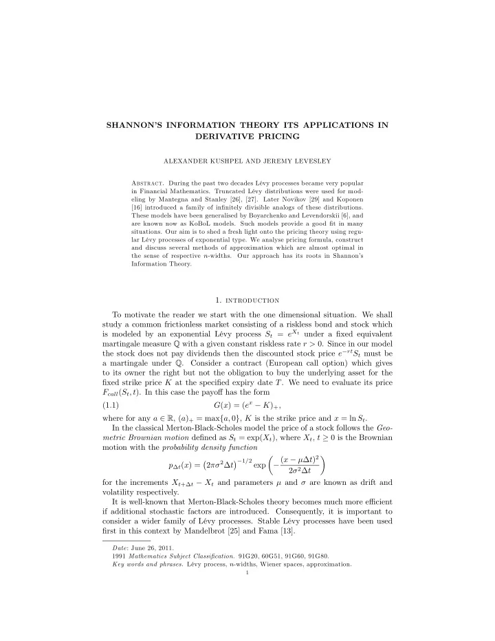
SHANNON’S INFORMATION THEORY ITS APPLICATIONS IN DERIVATIVE PRICING ALEXANDER KUSHPEL AND JEREMY LEVESLEY Abstract. During the past two decades Lévy processes became very popular in Financial Mathematics. Truncated Lévy distributions were used for mod- eling by Mantegna and Stanley [26], [27]. Later Novikov [29] and Koponen [16] introduced a family of in…nitely divisible analogs of these distributions. These models have been generalised by Boyarchenko and Levendorskii [6], and are known now as KoBoL models. Such models provide a good …t in many situations. Our aim is to shed a fresh light onto the pricing theory using regu- lar Lévy processes of exponential type. We analyse pricing formula, construct and discuss several methods of approximation which are almost optimal in the sense of respective n -widths. Our approach has its roots in Shannon’s Information Theory. 1. introduction To motivate the reader we start with the one dimensional situation. We shall study a common frictionless market consisting of a riskless bond and stock which is modeled by an exponential Lévy process S t = e X t under a …xed equivalent martingale measure Q with a given constant riskless rate r > 0 . Since in our model the stock does not pay dividends then the discounted stock price e � rt S t must be a martingale under Q . Consider a contract (European call option) which gives to its owner the right but not the obligation to buy the underlying asset for the …xed strike price K at the speci…ed expiry date T . We need to evaluate its price F call ( S t ; t ) . In this case the payo¤ has the form G ( x ) = ( e x � K ) + ; (1.1) where for any a 2 R , ( a ) + = max f a; 0 g , K is the strike price and x = ln S t . In the classical Merton-Black-Scholes model the price of a stock follows the Geo- metric Brownian motion de…ned as S t = exp( X t ) , where X t , t � 0 is the Brownian motion with the probability density function � � � � � 1 = 2 exp � ( x � � � t ) 2 2 �� 2 � t p � t ( x ) = 2 � 2 � t for the increments X t +� t � X t and parameters � and � are known as drift and volatility respectively. It is well-known that Merton-Black-Scholes theory becomes much more e¢cient if additional stochastic factors are introduced. Consequently, it is important to consider a wider family of Lévy processes. Stable Lévy processes have been used …rst in this context by Mandelbrot [25] and Fama [13]. Date : June 26, 2011. 1991 Mathematics Subject Classi…cation. 91G20, 60G51, 91G60, 91G80. Key words and phrases. Lévy process, n -widths, Wiener spaces, approximation. 1

2 ALEXANDER KUSHPEL AND JEREMY LEVESLEY From the 90th Lévy processes became very popular (see, e.g., [26], [27], [5], [6] and references therein). 2. basic definitions and results Let x ; y 2 R n , x = ( x 1 ; :::; x n ) ; y = ( y 1 ; :::; y n ) , x � y be the usual scalar product in R n , i.e., X n x � y = x k y k 2 R k =1 and j x j := ( x � x ) 1 = 2 : For a …nite measure � on R n we de…ne its Fourier transform as Z R n e � i x � y � ( d x ) b � ( y ) = F � ( y ) = and its formal inverse Z 1 � ( d x ) = F � 1 b R n e i x � y b � ( d x ) = � ( y ) d y : (2 � ) n It is known that if � is in…nitely divisible then there exists a unique continuous function � : R n ! C such that � ( 0 ) = 0 and e � ( y ) = b � ( y ) : Hence, the characteristic function of the distribution of X t of any Lévy process can be represented in the form � e i x � X t � = e � t ( x ) ; E where x 2 R n , t 2 R + and the function ( x ) is uniquely determined. This function is called the characteristic exponent . Vice versa, a Lévy process X = f X t g t 2 R + is determined uniquely by its characteristic exponent ( x ) . We say that a matrix A is nonnegative-de…nite (or positive-semide…nite) if x � A x � 0 for all x 2 C n (or for all x 2 R n for the real matrix), where x � is the conjugate transpose. A matrix A is nonnegative-de…nite if and only if it arises as the Gram matrix of some set of vectors v 1 ; � � � ; v n , i.e. A = ( a ij ) = v j � v i . The key role in our analysis plays the following classical result known as the Lévy-Khintchine formula which gives a representation of characteristic functions of all in…nitely divisible distributions. Theorem 1. Let X = f X t g t 2 R + be a Lévy process on R n . Then its characteristic exponent admits the representation Z � � ( y ) = � 1 1 � e i y � x + i y � x � D ( x ) (2.1) 2 A y � y � i b � y � �( d x ) ; R n where � D ( x ) is the characteristic function of D := f x 2 R n ; j x j � 1 g , A is a symmetric nonnegative-de…nite n � n matrix, b 2 R n and �( d x ) is a measure on R n such that Z (2.2) R n min f 1 ; x � x g �( d x ) < 1 ; �( f 0 g ) = 0 : � ( y ) = e ( y ) . Hence b

DERIVATIVE PRICING 3 The density of � is known as the Lévy density and A is the covariance matrix . In particular, if A = 0 (or A = ( a j;k ) 1 � j;k � n , a j;k = 0 ) then the Lévy process is a pure non-Gaussian process and if � = 0 the process is Gaussian . We say that the Lévy process has bounded variation if its sample paths have bounded variation on every compact time interval. A Lévy process has bounded variation i¤ A = 0 and Z R n min fj x j ; 1 g � ( d x ) < 1 ; � ( f 0 g ) = 0 (see, e.g., [4], p.15). The systematic exposition of the theory of Lévy processes can be found in [10], [11], [12], [31], [2], [28]. 3. characteristic exponents and density functions De…nition 1. We say that the process is purely discontinuous if A = ( a j;k ) , a j;k = 0 , 1 � j; k � n and b = 0 in (2.1). Consider the one-dimensional case. It follows from (2.1) that for a purely dis- continuous process ( � ) can be written as Z � � 1 � e i�x + i�x� [ � 1 ; 1] ( x ) (3.1) ( � ) = �( dx ) : R We shall be concerned just with purely discontinuous processes. Applying (3.1) we get the following representation for the density function p t ( y ) ; Z p t ( y ) = 1 e iy� E [ e i�X t ] d� 2 � R Z = F � 1 � e � t ( � ) � ( y ) = 1 e iy� � t ( � ) d� 2 � R � � Z Z � � = 1 1 � e i�x + i�x� [ � 1 ; 1] ( x ) (3.2) exp iy� � t �( dx ) d�: 2 � R R To …nd an explicit expression of the integral (3.2) we need to assume a very speci…c form of �( dx ) . Consequently, an explicit representations in this case is a real rarity. For instance, Barndor¤ and Nielsen [3] obtained the Lebesgue density function for generalised hyperbolic distributions which depends on …ve parameters � 2 � � 2 � �= 2 � � 2 + ( x � � ) 2 � ( � � 1 = 2) = 2 � d ( x; �; �; �; �; � ) = � � 2 � � 2 � (2 � ) 1 = 2 � � � 1 = 2 � � +1 K � � x � � 2 �� 1 = 2 � � � � 2 + 2 e � ( x � � ) ; � K � � 1 = 2 � where K � ( x ) is the modi…ed Bessel function of the third kind, Z 1 K � ( x ) = 1 � � � 1 e � x ( � � � � 1 ) = 2 d�: 2 0 Motivated by the idea to consider a wider class of models we need to decide at which stage we should fall into numerical methods. If we still want to be strapped with an explicit form of the characteristic exponent but still agree to apply numerical methods to compute the density function p t ( y ) then we apply the following standard trick. The sense of this manipulation is based on Cauchy’s theorem (see, e.g., [30]). Let T be the expiry date, t < T and G ( X T ) � 0 be the terminal payo¤ at the