SequenceAlignment September 6, 2018 1 Lecture 8: Sequence - PDF document
SequenceAlignment September 6, 2018 1 Lecture 8: Sequence Alignment CBIO (CSCI) 4835/6835: Introduction to Computational Biology 1.1 Overview and Objectives In our last lecture, we covered the basics of molecular biology and the role of
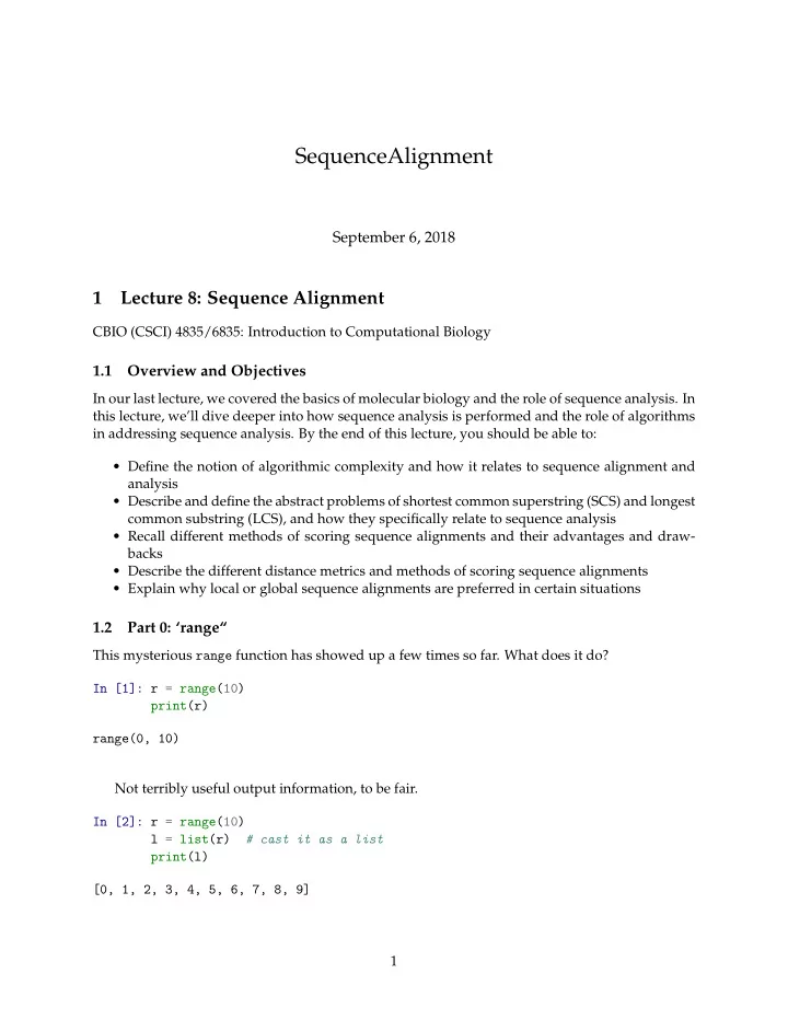
SequenceAlignment September 6, 2018 1 Lecture 8: Sequence Alignment CBIO (CSCI) 4835/6835: Introduction to Computational Biology 1.1 Overview and Objectives In our last lecture, we covered the basics of molecular biology and the role of sequence analysis. In this lecture, we’ll dive deeper into how sequence analysis is performed and the role of algorithms in addressing sequence analysis. By the end of this lecture, you should be able to: • Define the notion of algorithmic complexity and how it relates to sequence alignment and analysis • Describe and define the abstract problems of shortest common superstring (SCS) and longest common substring (LCS), and how they specifically relate to sequence analysis • Recall different methods of scoring sequence alignments and their advantages and draw- backs • Describe the different distance metrics and methods of scoring sequence alignments • Explain why local or global sequence alignments are preferred in certain situations 1.2 Part 0: ‘range“ This mysterious range function has showed up a few times so far. What does it do? In [1]: r = range(10) print(r) range(0, 10) Not terribly useful output information, to be fair. In [2]: r = range(10) l = list(r) # cast it as a list print(l) [0, 1, 2, 3, 4, 5, 6, 7, 8, 9] 1
range(i) generates a list of numbers from 0 (inclusive) to i (exclusive). This is very useful for looping! In [3]: for i in range(10): print(i) 0 1 2 3 4 5 6 7 8 9 You can also provide a second argument to range , which specifies a starting point for the count- ing (other than 0). That starting point is still inclusive , and the ending point still exclusive . In [4]: for i in range(5, 10): print(i) 5 6 7 8 9 Finally, you can also provide a third argument, which specifies the interval between numbers in the output. So far, that interval has been 1: start at 0, to go i , by ones. You can change that “by ones” to whatever you want. In [5]: for i in range(5, 10, 2): # read: from 5, to 10, by 2 print(i) 5 7 9 You can get really crazy with this third one, if you want: you can go backwards by putting in a negative interval. In [6]: for i in range(10, 0, -2): # from 10, to 0, by -2 print(i) 2
10 8 6 4 2 Same rules apply, though: the starting point is inclusive (hence why we see a 10), and the ending point is exclusive (hence why we don’t see a 0). range is particularly useful as a way of looping through a list of items by index . In [7]: list_of_interesting_things = [93, 17, 5583, 47, 2359875, 4, 381] for item in list_of_interesting_things: print(item, end = " ") 93 17 5583 47 2359875 4 381 This is how we’ve seen loops so far: the loop variable (here it’s item ) is a literal item in the list. But what if, in addition to the item, I needed to know where in the list that item was (i.e., the item’s list index)? In [8]: list_length = len(list_of_interesting_things) for index in range(list_length): # use range of the list length! item = list_of_interesting_things[index] # pull out the item AT that index print("Item " + str(item) + " at index " + str(index)) Item 93 at index 0 Item 17 at index 1 Item 5583 at index 2 Item 47 at index 3 Item 2359875 at index 4 Item 4 at index 5 Item 381 at index 6 1.3 Part 1: Complexity 1.3.1 Big “Oh” Notation From computer science comes this notion: how the runtime of an algorithm changes with respect to its input size. O ( n ) - the “ O ” is short for “order of the function”, and the value inside the parentheses is always with respect to n , interpreted to be the variable representing the size of the input data. 1.3.2 Limits Big-oh notation is a representation of limits, and most often we are interested in “worst-case” runtime. Let’s start with the example from the last lecture. 3
bigoh In [9]: a = [1, 2, 3, 4, 5] for element in a: print(element) 1 2 3 4 5 How many steps, or iterations, does this loop require to run? Alright, back to complexity: In [10]: a = range(100) for element in a: print(element, end = " ") 0 1 2 3 4 5 6 7 8 9 10 11 12 13 14 15 16 17 18 19 20 21 22 23 24 25 26 27 28 29 30 31 32 33 34 35 How many iterations does this loop require? For iterating once over any list using a single for loop, how many iterations does this re- quire? Algorithms which take n iterations to run, where n is the number of elements in our data set, are referred to as running in O ( n ) time. This is roughly interpreted to mean that, for n data points, n processing steps are required. Important to note : we never actually specify how much time a single processing step is. It could be a femtosecond, or an hour. Ultimately, it doesn’t matter. What does matter when something is O ( n ) is that, if we add one more data point ( n + 1), then however long a single processing step is, the algorithm should take only that much longer to run. How about this code? What is its big-oh? 4
In [11]: a = range(100) b = range(1, 101) for i in a: print(a[i] * b[i], end = " ") 0 2 6 12 20 30 42 56 72 90 110 132 156 182 210 240 272 306 342 380 420 462 506 552 600 650 702 756 Still O ( n ) . The important part is not (directly) the number of lists, but rather how we operate on them: again, we’re using only 1 for loop , so our runtime is directly proportional to how long the lists are. How about this code? In [12]: a = range(100) x = [] for i in a: x.append(i ** 2) for j in a: x.append(j ** 2) Trick question! One loop, as we’ve seen, is O ( n ) . Now we’ve written a second loop that is also O ( n ) , so literally speaking the runtime is 2 ∗ O ( n ) , but what happens to the 2 in the limit as n → ∞ ? The 2 is insignificant , so the overall big-oh for this code is still O ( n ) . How about this code? In [13]: a = range(100) for element_i in a: for element_j in a: print(element_i * element_j, end = " ") 0 0 0 0 0 0 0 0 0 0 0 0 0 0 0 0 0 0 0 0 0 0 0 0 0 0 0 0 0 0 0 0 0 0 0 0 0 0 0 0 0 0 0 0 0 0 0 0 0 Nested for loops are brutal–the inner loop runs in its entirety for every single iteration of the outer loop. In the limit, for a list of length n , there are O ( n 2 ) iterations. One more tricky one: In [14]: xeno = 100 while xeno > 1: xeno /= 2 print(xeno, end = " ") 50.0 25.0 12.5 6.25 3.125 1.5625 0.78125 Maybe another example from the same complexity class: In [15]: xeno = 100000 while xeno > 1: xeno /= 10 print(xeno, end = " ") 5
10000.0 1000.0 100.0 10.0 1.0 What does this “look” like? In [16]: # I'm just plotting the iteration number against the value of "xeno". %matplotlib inline import matplotlib.pyplot as plt x = [] y = [] xeno = 10000 i = 1 while xeno > 1: x.append(i) y.append(xeno) xeno /= 10 i += 1 plt.plot(x, y) Out[16]: [<matplotlib.lines.Line2D at 0x11e143c18>] In the first one, on each iteration, we’re dividing the remaining space by 2, halving again and again and again. In the second one, on each iteration, we’re dividing the space by 10. O ( log n ) . We use the default (base 10) because, in the limit, constants don’t matter. 6
1.4 Part 2: SCS and LCS Recall from the last lecture what SCS (shortest common superstring) was: • The shortest common superstring, given sequences X and Y , is the shortest possible se- quence that contains all the sequences X and Y . For example, let’s say we have X = ABACBDCAB and Y = BDCABA . What would be the shortest common superstring? Here is one alignment: BDCABA (second string) and ABACBDCAB (first string). The ABA is where the two strings overlap. The full alignment, BDCABACBDCAB , has a length of 12. Can we do better? ABACBDCAB and BDCAB A, which gives a full alignment of ABACBDCABA , which has a length of only 10. So this alignment would be the SCS. (When do we need to use SCS?) 1.4.1 Longest Common Substring (LCS) In a related, but different, problem: longest common substring asks: • Given sequences X and Y , the longest common substring is the constituent of the sequences X and Y that is as long as possible. Let’s go back to our sequences from before: X = ABACBDCAB and Y = BDCABA . What would be the longest common substring? The easiest substrings are the single characters A , B , C , and D , which both X and Y have. But these are short: only length 1 for all. Can we do better? ABACBDCAB and BDCAB A, so the longest common substring is BDCAB . (When do we need LCS?) 1.4.2 Rudimentary Sequence Alignment Given two DNA sequences v and w : v : ATATATAT w : TATATATA How would you suggest aligning these sequences to determine their similarity? Before we try to align them, we need some objective measure of what a “good” alignment is! 1.5 Part 3: Distance Metrics Hopefully, everyone has heard of Euclidean distance : this is the usual “distance” formula you use when trying to find out how far apart two points are in 2D space. How is it computed? For two points in 2D space, a and b , their Euclidean distance d e ( a , b ) is defined as: � ( a x − b x ) 2 + ( a y − b y ) 2 ) d e ( a , b ) = So if a = ( 1, 2 ) and b = ( 5, 3 ) , then: ( − 4 ) 2 + ( − 1 ) 2 = √ ( 1 − 5 ) 2 + ( 2 − 3 ) 2 = � � d e ( a , b ) = 16 + 1 = 4.1231 How can we measure distance between two sequences? 7
Recommend
More recommend
Explore More Topics
Stay informed with curated content and fresh updates.


![Lipschitz Quotients [S. Bates], W.B.J., J. Lindenstrauss, D. Preiss, G. Schechtman Background](https://c.sambuz.com/755604/lipschitz-quotients-s-bates-w-b-j-j-lindenstrauss-d-s.webp)
