Semaphores Dr. Liam OConnor University of Edinburgh LFCS (and UNSW) - PowerPoint PPT Presentation
Semaphores Producer-Consumer Semaphores Dr. Liam OConnor University of Edinburgh LFCS (and UNSW) Term 2 2020 1 Semaphores Producer-Consumer Where we are at In the last lecture, we saw more about hardware-assisted critical sections and
Semaphores Producer-Consumer Semaphores Dr. Liam O’Connor University of Edinburgh LFCS (and UNSW) Term 2 2020 1
Semaphores Producer-Consumer Where we are at In the last lecture, we saw more about hardware-assisted critical sections and how they are used to implement a basic unit of synchronisation, called a lock or mutex . In this lecture, we will generalise this concept to a semaphore with a particular analysis of the producer consumer problem . 2
Semaphores Producer-Consumer Semaphores Definition A semaphore can be abstractly viewed as a pair ( v , L ) of a natural number v and a set of processes L . The semaphore must always be initialised to some ( v , ∅ ). There are two basic operations a process p could perform on a semaphore S : wait ( S ) or P ( S ), decrements v if positive, otherwise adds p to L and blocks p . signal ( S ) or V ( S ), if L � = ∅ , unblocks a member of L . Otherwise increment v . Example (Promela Encoding) inline wait(S) { d_step { S > 0; S-- }} 1 inline signal(S) { d_step { S ++ } } 2 This is known as a busy-wait semaphore as the set L is implicitly the set of (busy-)waiting processes on the integer. 3
Semaphores Producer-Consumer Critical Sections Our previously mentioned locks are just semaphores where the integer starts at 1: p 2 q 2 (1 , ∅ ) semaphore S ← (1 , ∅ ) forever do forever do p 4 q 2 p 2 q 4 p 1 non-critical section q 1 non-critical section (0 , ∅ ) (0 , ∅ ) p 2 wait ( S ) q 2 wait ( S ); p 3 critical section q 3 critical section p 4 signal ( S ) q 4 signal ( S ); p 4 q 2 p 2 q 4 (0 , { q } ) (0 , { p } ) A weak semaphore is akin to our set model earlier. A busy-wait semaphore has no set, and implements blocking by spinning in a loop. Question What impact does weak vs. busy-wait have on eventual entry? 4
Semaphores Producer-Consumer For N processes semaphore S ← (1 , ∅ ) Problem 1: With a weak or busy-wait each process i: forever do semaphore we don’t satisfy eventual entry with- i 1 out a signal fairness assumption. non-critical section i 2 wait ( S ) Problem 2: Even with some kind of signal fair- i 3 critical section ness assumption, we don’t have linear waiting . i 4 signal ( S ) Strong Semaphores Replace the set L with a queue, such that processes are woken up in FIFO order. This guarantees linear waiting , but is of course harder to implement and potentially more expensive than our previous weak or busy-wait semaphores . 5
Semaphores Producer-Consumer Reasoning about Semaphores For a semaphore S = ( v , L ) initialised to ( k , ∅ ), the following invariants always hold: v = k + #signal( S ) − #wait( S ) 1 v ≥ 0 2 Definitions #signal( S ) is the number of times signal ( S ) has successfully executed. 1 #wait( S ) is the number of times wait ( S ) has successfully executed. 2 Here we define successful execution to mean that the process has proceeded to the following statement. So if a process is blocked on a wait ( S ), then #wait( S ) will not increase until the process is unblocked. Example (Mutual Exclusion) Observe the invariant that the no. of processes in their CS = #wait( S ) − #signal( S ). Let’s use this to show our usual properties. 6
Semaphores Producer-Consumer Safety Properties Mutual Exclusion We know: v = 1 + #signal( S ) − #wait( S ) (our first semaphore invariant) 1 v ≥ 0 (our second semaphore invariant) 2 #CS = #wait( S ) − #signal( S ) (our observed invariant) 3 From these invariants it is possible to show that #CS ≤ 1, i.e. mutual exclusion. Absence of Deadlock Assume that deadlock occurs by all processes being blocked on wait , so no process can enter its critical section (#CS = 0). Then v = 0, contradicting our semaphore invariants above. So there cannot be deadlock. 7
Semaphores Producer-Consumer Liveness Properties To simplify things, we will prove for only two processes, p and q . Eventual Entry for p Assume that p is starved, indefinitely blocked on the wait .Therefore S = (0 , L ) and p ∈ L . We know therefore, substituting into our invariants: 0 = 1 + #signal( S ) − #wait( S ) 1 #CS = #wait( S ) − #signal( S ) 2 From which we can conclude that #CS = 1.Therefore q must be in its critical section and L = { p } . By a progress assumption a , we know that eventually q will finish its CS and signal ( S ). Thus, p will be unblocked, causing it to gain entry — Contradiction . a Merely that processes that are able to move will do so when asked by the scheduler. 8
Semaphores Producer-Consumer Rendezvous In addition (and perhaps simpler) than the mutual exclusion/critical section problem, the rendezvous problem is also a basic unit of synchronisation for solving concurrency problems. Assume we have two processes with two statements each: Rendezvous P Q first P first Q second P second Q Problem How do we ensure that all first statements happen before all second statements? On iPad 9
Semaphores Producer-Consumer Producer-Consumer So-called binary semaphores (locks) are not the only use of semaphores! Producer-Consumer Problem A producer process and a consumer process share access to a shared buffer of data. This buffer acts as a queue. The producer adds messages to the queue, and the consumer reads messages from the queue. If there are no messages in the queue, the consumer blocks until there are messages. Algorithm 1.1: Producer-consumer (infinite buffer) queue[T] buffer ← empty queue; semaphore full ← (0 , ∅ ) producer consumer T d T d forever do forever do d ← produce wait (full) p1: q1: append(d, buffer) d ← take(buffer) p2: q2: signal (full) consume(d) p3: q3: 10
Semaphores Producer-Consumer Finite buffer What about if the buffer can become full, and the producer must block until space is freed? Use another semaphore! : Algorithm 1.2: Producer-consumer (finite buffer, semaphores) bounded[N] queue[T] buffer ← empty queue semaphore full ← (0 , ∅ ) semaphore empty ← ( N , ∅ ) producer consumer T d T d loop forever loop forever d ← produce wait (full) p1: q1: d ← take(buffer) wait (empty) p2: q2: append(d, buffer) signal (empty) p3: q3: signal (full) consume(d) p4: q4: This pattern is called split semaphores . 11
Semaphores Producer-Consumer A specific Example Algorithm 1.3: Producer/Consumer ( b -place buffer, sem’s) integer data[ b ] semaphore empty ← ( b , ∅ ), full ← (0 , ∅ ) producer consumer integer i ← 0 integer k ← 0, t ← 0 loop forever loop forever wait(empty) wait(full) p1: q1: data[i % b ] ← g (i) t ← t + data[k % b ] p2: q2: i ++ k ++ p3: q3: signal(full) signal(empty) p4: q4: 12
Semaphores Producer-Consumer What do we prove? The crucial properties of this pair of processes include: � � t = � k − 1 safety S = j =0 g ( j ) is an invariant liveness k keeps increasing 13
Semaphores Producer-Consumer How do we prove? To show the safety property, we translate the pseudo code into transition diagrams, 1 define a pre-condition φ 2 define an assertion network Q , 3 prove that Q is (a) inductive and (b) interference-free, 4 prove that the initial assertions Q p1 and Q q1 follow from φ , and 5 prove that each of the consumer’s assertions implies the invariant S . 6 14
Semaphores Producer-Consumer 1 Transition Diagrams e > 0 → e -- f > 0 → f -- p1 p2 q1 q2 e ++ f ++ data [ i % b ] , i ← t , k ← g ( i ) , i + 1 t + data [ k % b ] , k + 1 p4 q4 15
Semaphores Producer-Consumer 2 Precondition As precondition we collect the initial values of those global and local variables which are read before they are written. φ = ( e = b ∧ f = 0 ∧ i = k = t = 0) 16
Semaphores Producer-Consumer 3 Assertion Network I We start by collecting further likely invariants. The consumer can’t overtake the producer: 0 ≤ k ≤ i (1) The producer can’t lap the consumer: i − k ≤ b (2) The buffer shows a subsequence of g ’s values: ∀ j ∈ a .. i − 1 ( data [ j % b ] = g ( j )) , where a = max(0 , i − b ) (3) 17
Semaphores Producer-Consumer 3 Assertion Network II semaphore invariants: e , f ∈ 0 .. b (4) e = b + #signal( e ) − #wait( e ) (5) f = #signal( f ) − #wait( f ) (6) numbers of waits and signals are correlated: #wait( e ) = #signal( f ) + 1 − p 1 = i + p 2 (7) #signal( f ) = #wait( e ) − p 2 , 4 = i − p 4 (8) #wait( f ) = #signal( e ) + 1 − q 1 = k + q 2 (9) #signal( e ) = #wait( f ) − q 2 , 4 = k − q 4 (10) 18
Semaphores Producer-Consumer 3 Assertion Network III semaphore values are correlated: e + f = b − p 2 , 4 − q 2 , 4 (11) our goal: (12) S Assuming that the invariants (1)–(12) gather all that’s going on we may now try to prove that the assertion network consisting of the same assertion, I = (1) ∧ . . . ∧ (12) at every location is inductive and interference-free. 19
Semaphores Producer-Consumer 4(a) Q is inductive We need to prove local correctness of each of the 6 transitions. We assume that the auxiliary variables p 1 , p 2 , p 4 , q 1 , q 2 , and q 4 are implicitly set to 0 resp. 1, depending on the locations. p1 → p2: | = I ∧ e > 0 = ⇒ I ◦ ( e ← e − 1) (13) p2 → p4: | = I = ⇒ I ◦ ( data [ i % b ] , i ← g ( i ) , i + 1) (14) p4 → p1: | = I = ⇒ I ◦ ( f ← f + 1) (15) q1 → q2: | = I ∧ f > 0 = ⇒ I ◦ ( f ← f − 1) (16) q2 → q4: | = I = ⇒ I ◦ ( t , k ← t + data [ k % b ] , i + 1) (17) q4 → q1: | = I = ⇒ I ◦ ( e ← e + 1) (18) 20
Recommend
More recommend
Explore More Topics
Stay informed with curated content and fresh updates.
