Sectoral vs. Aggregate Shocks: A Structural Factor Analysis of - PowerPoint PPT Presentation

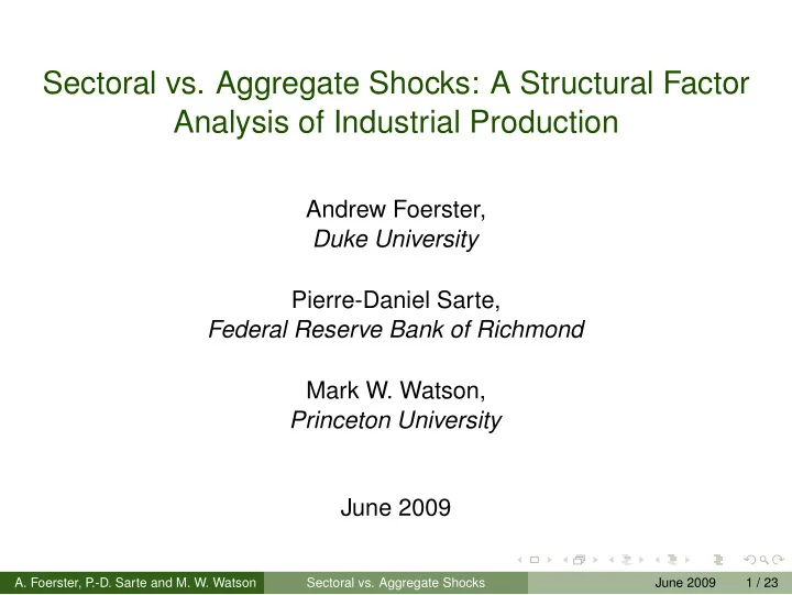
Sectoral vs. Aggregate Shocks: A Structural Factor Analysis of Industrial Production Andrew Foerster, Duke University Pierre-Daniel Sarte, Federal Reserve Bank of Richmond Mark W. Watson, Princeton University June 2009 A. Foerster, P .-D. Sarte and M. W. Watson Sectoral vs. Aggregate Shocks () June 2009 1 / 23

Observations and Motivating Questions Month-to-month and quarter-to-quarter variations in Industrial Production (IP) are large ◮ std. dev. of monthly growth rates is 8 percent ◮ std. dev. of quarterly growth rates is 6 percent ◮ noticeably large fall in the volatility of IP after 1984 IP index is constructed as a weighted average of production indices across a large number of sectors... ... apparently, much of the variability in individual sectors does not “average out” A. Foerster, P .-D. Sarte and M. W. Watson Sectoral vs. Aggregate Shocks () June 2009 2 / 23

An Initial Look at IP Data A. Foerster, P .-D. Sarte and M. W. Watson Sectoral vs. Aggregate Shocks () June 2009 3 / 23

Observations and Motivating Questions Aggregate Shocks that affect all industrial sectors Some sectors have very large weights in the aggregate index, Gabaix (2005) Complementarities in production amplify and propagate sector-specific shocks ◮ input-output (IO) linkages ◮ aggregate activity spillovers ◮ local activity spillovers A. Foerster, P .-D. Sarte and M. W. Watson Sectoral vs. Aggregate Shocks () June 2009 4 / 23

Approaches to analyzing sources of variations in the business cycle Factor Analytic Methods - Long and Plosser (1987), Forni and Reichlin (1998), Shea (2002) ◮ broad identifying restrictions ◮ Non-trivial contribution of sector-specific shocks to aggregate variability (approximately 50 percent) Structural (calibrated) Models - Long and Plosser (1983), Horvath (1998), Dupor (1999), Horvath (1998, 2000) ◮ contribution of idiosyncratic shocks to aggregate variability depends on exact structure of IO matrix Other: Conley and Dupor (2003), Gabaix (2005), Comin and Philippon (2005) A. Foerster, P .-D. Sarte and M. W. Watson Sectoral vs. Aggregate Shocks () June 2009 5 / 23

Overview for this paper Bridge factor-analytic and structural approaches to the analysis of idiosyncratic and aggregate shocks ◮ Highlight conditions under which multisector growth models (Long and Plosser 1983, Horvath 1998) produce factor models as reduced forms ◮ Factors are associated with aggregate productivity shocks ◮ “Uniquenesses” are associated with (linear combinations of) sector-specific productivity shocks Sort through leading explanations underlying: ◮ both aggregate and sectoral IP volatility ◮ the decline in aggregate IP volatility after 1984 A. Foerster, P .-D. Sarte and M. W. Watson Sectoral vs. Aggregate Shocks () June 2009 6 / 23

Std. Dev. of Sectoral IP Growth Rates A. Foerster, P .-D. Sarte and M. W. Watson Sectoral vs. Aggregate Shocks () June 2009 7 / 23

Standard Deviation of IP Growth Rates (Percentage points at annual rate) Share Weights Used to Monthly Growth Rates Quarterly Growth Rates Aggregate Sectoral IP 1972- 1972- 1984- 1972- 1972- 1984- 2007 1983 2007 2007 1983 2007 a. Full Covariance Matrix of Sectoral Growth Rates Time Varying ( w it ) 8.3 11.6 6.2 5.8 8.7 3.6 Constant ( µ w ) 8.4 11.7 6.2 5.8 8.9 3.6 Equal (1 / N ) 10.4 14.4 7.6 6.9 10.5 4.2 b. Diagonal Covariance Matrix of Sectoral Growth Rates Time Varying ( w it ) 4.3 4.9 4.1 1.9 2.6 1.6 Constant ( µ w ) 4.2 4.6 4.0 1.9 2.4 1.5 Equal (1 / N ) 4.6 5.6 4.0 1.8 2.5 1.4 A. Foerster, P .-D. Sarte and M. W. Watson Sectoral vs. Aggregate Shocks () June 2009 8 / 23

Statistical Factor Analysis X t = Λ F t + u t X t is an Nx1 vector of sectoral output growth rates, F t is a set of r common factors, and u t is an Nx1 vector of idiosyncratic disturbances that satisfy weak dependence Principle components of X t are consistent estimators of F t , Stock and Watson (2002) - Bai and Ng (2002) yield 1 or 2 factors g t = w ′ X t = w ′ Λ F t + w ′ u t R 2 ( F ) = w ′ ΛΣ FF Λ ′ w / σ 2 g Distribution of R 2 i ( F ) A. Foerster, P .-D. Sarte and M. W. Watson Sectoral vs. Aggregate Shocks () June 2009 9 / 23

Statistical Factor Analysis Decomposition of Variance from Statistical 2-Factor Model Monthly Rates Quarterly Rates 72-83 84-07 72-83 84-07 Std. Deviation of IP Growth Rates Implied by Factor Model 11.7 6.2 8.9 3.6 (with Constant Share Weights) R 2 ( F ) 0.86 0.49 0.89 0.87 A. Foerster, P .-D. Sarte and M. W. Watson Sectoral vs. Aggregate Shocks () June 2009 10 / 23

Distribution of R 2 i ( F ) of Sectoral Growth Rates A. Foerster, P .-D. Sarte and M. W. Watson Sectoral vs. Aggregate Shocks () June 2009 11 / 23

Information Content of IP Contained in Individual Sectors Selected Sectors 1972-1983 1984-2000 Ranked by R 2 i ( F ) Fraction of Explained IP Fraction of Explained IP Top 5 Sectors 85.0 75.4 Top 10 Sectors 90.3 80.4 Top 20 Sectors 97.9 86.4 Top 30 Sectors 98.8 90.3 A. Foerster, P .-D. Sarte and M. W. Watson Sectoral vs. Aggregate Shocks () June 2009 12 / 23

Structural Factor Analysis Consistent estimation of factors relies on weak cross-sectional dependence of “uniquenesses”, u t ... ... but IO linkages can transform sector-specific shocks into common shocks Require a model that incorporates linkages across sectors - Long and Plosser (1983), Horvath (1998) Key feature is that production in each sector uses materials produced in other sectors Statistical Factor Model can be interpreted as the reduced form of the Structural Model. We can filter out the effects of IO linkages. A. Foerster, P .-D. Sarte and M. W. Watson Sectoral vs. Aggregate Shocks () June 2009 13 / 23

Structural Factor Analysis N distinct sectors, indexed j = 1 ,..., N Technology: N 1 − α j − ∑ N γ ij i = 1 γ ij α j ∏ Y jt = A jt K M ij L jt jt , i = 1 M ij - quantity of sector i material used in sector j . An input-output matrix for this economy is an N x N matrix, Γ , with typical element γ ij N + 1 disturbances ∆ lnA jt = ǫ jt ǫ t = ( ǫ 1 t , ǫ 2 t ,..., ǫ Nt ) ′ has covariance matrix Σ ǫǫ A. Foerster, P .-D. Sarte and M. W. Watson Sectoral vs. Aggregate Shocks () June 2009 14 / 23

Structural Factor Analysis preferences: C 1 − σ ∞ N jt β t ∑ ∑ E ( 1 − σ − ψ L jt ) t = 0 j = 1 resource constraints: N ∑ C jt + M jit + K jt + 1 − ( 1 − δ ) K jt = Y jt , j = 1 ,..., N i = 1 Planner’s solution for sectoral output allocations, X t = Φ X t − 1 + Π ǫ t + Ξ ǫ t − 1 , where X t = ( ∆ ln ( Y 1 t ) , ∆ ln ( Y 2 t ) ,..., ∆ ln ( Y Nt )) ′ Φ , Π , and Ξ are N × N matrices that depend only on the model parameters, α d , Γ , β , σ , ψ , and δ A. Foerster, P .-D. Sarte and M. W. Watson Sectoral vs. Aggregate Shocks () June 2009 15 / 23

Structural Factor Analysis ǫ t = Λ s S t + v t , where v t has a diagonal variance-covariance matrix then X t = Λ F t + u t , where Λ ( L ) = ( I − Φ L ) − 1 ( Π + Ξ L ) Λ s , F t = S t , and u t = ( I − Φ L ) − 1 ( Π + Ξ L ) v t The structural model produces a an approximate factor model as a reduced form. Common factors are associated with aggregate shocks to sectoral productivity. “Uniquenesses” are linear combinations of the sector-specific shocks. A. Foerster, P .-D. Sarte and M. W. Watson Sectoral vs. Aggregate Shocks () June 2009 16 / 23

Structural Factor Analysis Special case, Horvath (1998), Dupor (1999): no labor, full depreciation, and log preferences The model’s exact solution is given by Φ = ( I − Γ ′ ) − 1 α d , Ξ = 0, and Π = ( I − Γ ′ ) − 1 so that ′ ) − 1 α d L ) − 1 ( I − Γ ′ ) − 1 v t u t = ( I − ( I − Γ To eliminate the propagation of sector-specifc shocks induced by IO linkages, filter the vector of sectoral output growth ǫ t = ( Π + Ξ L ) − 1 ( I − Φ L ) X t A. Foerster, P .-D. Sarte and M. W. Watson Sectoral vs. Aggregate Shocks () June 2009 17 / 23

Largest Eigenvalues of Sample Correlation Matrix IO Model with Uncorrelated Sector-Specific Shocks a. NAICS (1998 IO Matrix) 1972-1983 1984-2007 Eigenvalue Model %-tiles Model %-tiles Rank Data 1 50 99 Data 1 50 99 1 39.4 6.6 8.0 10.1 18.5 4.7 5.5 6.7 2 11.0 5.8 6.4 7.3 6.7 4.1 4.5 5.0 3 5.9 5.3 5.8 6.3 5.1 3.8 4.1 4.5 4 4.8 5.0 5.4 5.8 4.4 3.6 3.8 4.1 5 4.6 4.7 5.0 5.4 4.1 3.5 3.7 3.9 6 4.1 4.5 4.8 5.1 3.6 3.3 3.5 3.7 7 3.5 4.2 4.5 4.8 3.4 3.2 3.4 3.5 A. Foerster, P .-D. Sarte and M. W. Watson Sectoral vs. Aggregate Shocks () June 2009 18 / 23

Largest Eigenvalues of Sample Correlation Matrix IO Model with 2 Factors for Sector-Specific Shocks a. NAICS (1998 IO Matrix) 1972-1983 1984-2007 Eigenvalue Model %-tiles Model %-tiles Rank Data 1 50 99 Data 1 50 99 1 39.4 30.1 39.7 48.4 18.5 14.9 19.2 23.6 2 11.0 8.4 12.2 16.9 6.7 6.3 8.3 10.6 3 5.9 3.6 4.2 5.0 5.1 3.4 3.8 4.4 4 4.8 3.3 3.7 4.3 4.4 3.2 3.5 3.8 5 4.6 3.0 3.5 3.9 4.1 3.0 3.2 3.5 6 4.1 2.8 3.2 3.7 3.6 2.8 3.1 3.3 7 3.5 2.7 3.0 3.4 3.4 2.7 2.9 3.1 A. Foerster, P .-D. Sarte and M. W. Watson Sectoral vs. Aggregate Shocks () June 2009 19 / 23