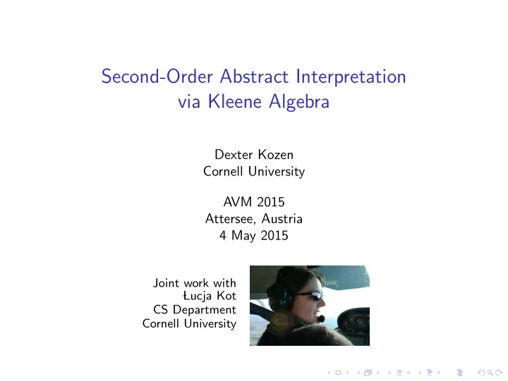
Second-Order Abstract Interpretation via Kleene Algebra Dexter - PowerPoint PPT Presentation

Second-Order Abstract Interpretation via Kleene Algebra Dexter Kozen Cornell University AVM 2015 Attersee, Austria 4 May 2015 Joint work with � Lucja Kot CS Department Cornell University

Abstract Interpretation Cousot & Cousot 79 ◮ Static derivation of information about the execution state at various points in a program ◮ Comes in various flavors ◮ type inference ◮ dataflow analysis ◮ set constraints ◮ Applications ◮ code optimization ◮ verification ◮ generating proof artifacts for PCC

Standard Approach ◮ Start with the control flow graph of the program to be analyzed ◮ Propagate known information forward – possible values of variables or types ◮ Compute a join at confluence points ◮ Standard method is called the worklist algorithm ◮ The process is a bit like running the program on abstract values, hence the name abstract interpretation

Types or Abstract Values ◮ Represent sets of values ◮ statically derivable ◮ conservative approximation ◮ Form a partial semilattice ◮ higher = less specific ◮ join does not exist = type error ◮ Often, abstract values are associated with invariants

This Talk ◮ A general mechanism for abstract interpretation and dataflow analysis based on Kleene algebra ◮ May improve performance over standard worklist algorithm when the semilattice of types is small ◮ Illustration of the method in the context of Java bytecode verification

Kleene Algebra (KA) (0 + 1(01 ∗ 0) ∗ 1) ∗ { multiples of 3 in binary } 1 0 1 0 0 1 ( ab ) ∗ a = a ( ba ) ∗ { a , aba , ababa , . . . } a b ( a + b ) ∗ = a ∗ ( ba ∗ ) ∗ { all strings over { a , b }} Stephen Cole Kleene a + b (1909–1994)

Foundations of the Algebraic Theory J. H. Conway. Regular Algebra and Finite Machines . Chapman and Hall, London, 1971. John Horton Conway (1937–)

Axioms of KA Idempotent Semiring Axioms p + ( q + r ) = ( p + q ) + r p ( qr ) = ( pq ) r p + q = q + p 1 p = p 1 = p p + 0 = p p 0 = 0 p = 0 p + p = p def p ( q + r ) = pq + pr a ≤ b ⇐ ⇒ a + b = b ( p + q ) r = pr + qr Axioms for ∗ 1 + pp ∗ ≤ p ∗ q + px ≤ x ⇒ p ∗ q ≤ x q + xp ≤ x ⇒ qp ∗ ≤ x 1 + p ∗ p ≤ p ∗

Significance of the ∗ Axioms 1 + pp ∗ ≤ p ∗ ⇒ q + pp ∗ q ≤ p ∗ q q + px ≤ x ⇒ p ∗ q ≤ x p ∗ q is the least x such that q + px ≤ x

Standard Model Regular sets of strings over Σ A + B = A ∪ B = { xy | x ∈ A , y ∈ B } AB A 0 ∪ A 1 ∪ A 2 ∪ · · · � A ∗ A n = = n ≥ 0 1 = { ε } 0 = ∅ This is the free KA on generators Σ

Relational Models Binary relations on a set X For R , S ⊆ X × X , R + S = R ∪ S RS = R ◦ S = { ( u , v ) | ∃ w ( u , w ) ∈ R , ( w , v ) ∈ S } R ∗ = reflexive transitive closure of R R 0 ∪ R 1 ∪ R 2 ∪ · · · � R n = = n ≥ 0 1 = identity relation = { ( u , u ) | u ∈ X } 0 = ∅ KA is complete for the equational theory of relational models

Other Models ◮ Trace models used in semantics ◮ (min , +) algebra used in shortest path algorithms ◮ (max , · ) algebra used in coding ◮ Convex sets used in computational geometry [Iwano & Steiglitz 90]

Matrices over a KA form a KA � a � e � a + e � � � b f b + f + = c d g h c + g d + h � � � � � � a b e f ae + bg af + bh · = c d g h ce + dg cf + dh � 0 � 1 � � 0 0 0 = 1 = 0 0 0 1 � ( a + bd ∗ c ) ∗ � a � ∗ ( a + bd ∗ c ) ∗ bd ∗ � b = ( d + ca ∗ b ) ∗ ca ∗ ( d + ca ∗ b ) ∗ c d b a d c

Systems of Affine Linear Inequalities Theorem Any system of n linear inequalities in n unknowns has a unique least solution q 1 + p 11 x 1 + p 12 x 2 + · · · p 1 n x n ≤ x 1 . . . q n + p n 1 x 1 + p n 2 x 2 + · · · p nn x n ≤ x n q 1 x 1 x 1 q 2 x 2 x 2 . . . + P = p ij ≤ . . . . . . q n x n x n Least solution is P ∗ q

Proof Artifacts An independently verifiable representation of the proof x ≤ y ⇒ x* ≤ y* λ x,y. λ P0.(trans< [y=x*;1 x=x* z=y*] (=< [x=x* y=x*;1] (sym [x=x*;1 y=x*] (id.R [x=x*])),*R [x=x y=1 z=y*] (trans< [y=1 + y;y* x=x;y* + 1 z=y*] (trans< [y=y;y* + 1 x=x;y* + 1 z=1 + y;y*] (mono+R [x=x;y* y=y;y* z=1] (mono.R [x=x y=y z=y*] P0), =< [x=y;y* + 1 y=1 + y;y*] (commut+ [x=y;y* y=1])), =< [x=1 + y;y* y=y*] (unwindL [x=y])))))

Example: Java Bytecode Verification Useless Object Integer Continuations int,short,byte, boolean,char Interface · · · Array[ ] Array[ ][ ] implements Java class hierarchy Null

Example: Java Bytecode Verification Typical bytecode instructions: iload 3 load an int from local 3, push on the operand stack istore 3 pop an int from the operand stack, store in local 3 iadd add the two ints on top of the stack, leave result on stack load a ref from local 4, push on the operand stack aload 4 pop a ref from the operand stack, store in local 4 astore 4 swap the two values on top of the stack (polymorphic) swap

Example: Java Bytecode Verification local variable array maxLocals Hash- String Object table this p 0 p 1 p 2 parameters other locals operand stack maxStack String- User- int[ ] Buffer Class integer reference continuation useless

A Directed Graph ◮ Vertices are instruction instances ◮ Edges to successor instructions, statically determined ◮ fallthrough ◮ jump targets ◮ exception handlers ◮ Edges labeled with transfer functions ◮ partial functions types → types ◮ models abstract effect of instruction ◮ domain of definition gives precondition for safe execution ◮ different successors may have different transfer functions

Example of a Transfer Function locals 0 1 2 3 4 5 6 7 ◮ Preconditions for safe stack execution ◮ local 3 is an integer iload 3 ◮ stack is not full ◮ Effect locals ◮ push integer in local 3 on stack 0 1 2 3 4 5 6 7 stack

Different exiting edges ⇒ different transfer functions fallthrough pop object; instruction pop field reference; push value object � = null getfield object = null dump stack; push NullPointerException exception handler

Abstract Interpretation locals stack ◮ Annotate each vertex with a type ◮ reflects best knowledge of the state immediately prior to execution of the instruction ◮ must satisfy preconditions of exiting transfer functions ◮ Annotation of the entry instruction is determined by the declared type of the method ◮ Annotation of other instructions = join of values of transfer functions applied to predecessors annotations ◮ Want least fixpoint = best conservative approximation

Example locals stack locals iload 3 stack locals stack iload 4 goto locals stack iadd locals locals stack stack istore 3

Example locals stack reference locals iload 3 stack locals stack iload 4 goto locals stack iadd integer useless locals locals stack stack istore 3

Example locals stack StringBuffer locals iload 3 stack locals stack iload 4 goto locals stack iadd String Object locals locals stack stack istore 3

Basic Worklist Algorithm ◮ Annotate entry instruction according to declared type of the method, put on worklist ◮ first n + 1 locals contain this , method parameters ◮ stack is empty ◮ Repeat until worklist is empty: ◮ remove next instruction from worklist ◮ for each exiting edge: ◮ apply transfer function on that edge to current annotation ◮ update successor annotation – join of transfer function value and current successor annotation ◮ join does not exist ⇒ type error ◮ if successor changed, put on worklist

An Application of Kleene Algebra ◮ Idea: avoid retracing of long cycles by symbolic composition of transfer functions ◮ Elements of the Kleene algebra are (typed) transfer functions ◮ multiplication = typed composition ◮ addition = join in the type semilattice ◮ Least fixpoint calculation involves computing the * of an m × m matrix, where m is the size of a cutset (set of vertices breaking all cycles)

Semilattices and the ACC ◮ Let ( L , + , ⊥ ) be a semilattice satisfying the ascending chain condition (ACC) x + ( y + z ) = ( x + y ) + z x + ⊥ = x x + y = y + x x + x = x ◮ ACC = no infinite ascending chains in L ◮ Implies that L contains a maximum element ⊤ ◮ Elements of L represent dataflow information ◮ lower = more information ◮ higher = less information ◮ ⊤ = no information

A Partial Order ◮ There is a natural partial order def x ≤ y ⇐ ⇒ x + y = y ◮ x + y is the least upper bound of x and y with respect to ≤

Transfer Functions ◮ Transfer functions are modeled as strict, monotone functions f : L → L ◮ monotone: x ≤ y ⇒ f ( x ) ≤ f ( y ) ◮ strict: f ( ⊥ ) = ⊥ ◮ Examples: 0 = λ x . ⊥ , 1 = λ x . x ◮ The domain of f is dom f = { x ∈ L | f ( x ) � = ⊤} ◮ monotonicity implies dom( f ) closed downward under ≤

Join ◮ Define a join operation on transfer functions: ( f + g )( x ) = f ( x ) + g ( x ) ◮ 0 = λ x . ⊥ is a two-sided identity for + (( λ x . ⊥ ) + g )( x ) = ⊥ + g ( x ) = g ( x ) ◮ idempotent f + f = f , thus we have a natural partial order def f ≤ g ⇐ ⇒ f + g = g ◮ upper semilattice with least element 0 = λ x . ⊥