Searching for Periodic Gene Expression Patterns Using Lomb-Scargle - PDF document

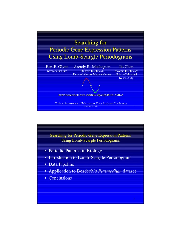
Searching for Periodic Gene Expression Patterns Using Lomb-Scargle Periodograms Earl F. Glynn Arcady R. Mushegian Jie Chen Stowers Institute Stowers Institute & Stowers Institute & Univ. of Kansas Medical Center Univ. of Missouri Kansas City http://research.stowers-institute.org/efg/2004/CAMDA Critical Assessment of Microarray Data Analysis Conference 1 November 11, 2004 Searching for Periodic Gene Expression Patterns Using Lomb-Scargle Periodograms • Periodic Patterns in Biology • Introduction to Lomb-Scargle Periodogram • Data Pipeline • Application to Bozdech’s Plasmodium dataset • Conclusions 2 1

Periodic Patterns in Biology A vertebrate’s body plan: a segmented pattern. Segmentation is established during somitogenesis. Photograph taken at Reptile Gardens, Rapid City, SD www.reptile-gardens.com 3 Periodic Patterns in Biology Intraerythrocytic Developmental Cycle of Plasmodium falciparum From Bozdech, et al, Fig. 1A, PLoS Biology , Vol 1, No 1, Oct 2003, p 3. Cy5 RNA from parasitized red blood cells Expression Ratio = = RNA from all development cycles Cy3 Values for Log 2 (Expression Ratio) are approximately normally distributed. Assume gene expression reflects observed biological periodicity. 4 2

Simple Periodic Gene Expression Model “On” “On” “On” 1 period period frequency = (T) (T) period Expression f = 1 T “Off” ω = angular frequency = 2 π f “Off” Time Gene Expression = Constant × Cosine(2 π f t) “Periodic” if only observed over a single cycle? 5 Introduction to Lomb-Scargle Periodogram • What is a Periodogram? • Why Lomb-Scargle Instead of Fourier? • Example Using Cosine Expression Model • Mathematical Details • Mathematical Experiments - Single Dominant Frequency - Multiple Frequencies - Mixtures: Signal and Noise 6 3

What is a Periodogram? • A graph showing frequency “power” for a spectrum of frequencies • “Peak” in periodogram indicates a frequency with significant periodicity Periodic Signal Periodogram Computation Spectral Log 2 (Expression) “Power” Frequency Time 7 Why Lomb-Scargle Instead of Fourier? • Missing data handled naturally • No data imputation needed • Any number of points can be used • No need for 2 N data points like with FFT • Lomb-Scargle periodogram has known statistical properties Note: The Lomb-Scargle algorithm is NOT equivalent to the conventional periodogram analysis based 8 Fourier analysis. 4

Lomb-Scargle Periodogram Example Using Cosine Expression Model Cosine Curve (N=48) A small value 1.0 for the false-alarm 0.5 Expression probability indicates 0.0 a highly significant -1.0 periodic signal. N = 48 0 10 20 30 40 Time [hours] Normalized Power Spectral Density Lomb-Scargle Periodogram Peak Significance Period at Peak = 48 hours p = 3.3e-009 at Peak T = 1 0.8 20 Probability p = 1e-06 f p = 1e-05 p = 1e-04 0.4 10 p = 0.001 p = 0.01 p = 0.05 5 0.0 0 0.00 0.05 0.10 0.15 0.20 0.00 0.05 0.10 0.15 0.20 Frequency [1/hour] Frequency [1/hour] 9 Evenly-spaced time points Lomb-Scargle Periodogram Example Using Noisy Cosine Expression Model Cosine Curve + Noise (N=48) Time Interval Variability 1.0 8 Expression Frequency 6 0.0 4 2 -1.0 0 N = 48 0 10 20 30 40 -1.0 -0.5 0.0 0.5 1.0 Time [hours] log10(delta T) Normalized Power Spectral Density Lomb-Scargle Periodogram Peak Significance Period at Peak = 45.7 hours p = 2.54e-007 at Peak 0.8 20 p = 1e-06 Probability p = 1e-05 p = 1e-04 0.4 10 p = 0.001 p = 0.01 p = 0.05 5 0.0 0 0.00 0.05 0.10 0.15 0.20 0.00 0.05 0.10 0.15 0.20 Frequency [1/hour] Frequency [1/hour] 10 Unevenly-spaced time points 5

Lomb-Scargle Periodogram Example Using Noise Noise (N=48) Time Interval Variability 1.0 8 0.5 Expression Frequency 6 0.0 4 2 -1.0 0 N = 48 0 10 20 30 40 -1.0 -0.5 0.0 0.5 1.0 Time [hours] log10(delta T) Normalized Power Spectral Density Lomb-Scargle Periodogram Peak Significance Period at Peak = 7.4 hours p = 0.973 at Peak 0.8 20 Probability p = 1e-06 p = 1e-05 p = 1e-04 0.4 10 p = 0.001 p = 0.01 p = 0.05 5 0.0 0 0.00 0.05 0.10 0.15 0.20 0.00 0.05 0.10 0.15 0.20 Frequency [1/hour] Frequency [1/hour] 11 Lomb-Scargle Periodogram Mathematical Details P N ( ω ) has an exponential probability distribution with unit mean. Source: Numerical Recipes in C (2 nd Ed), p. 577 12 6

Mathematical Experiment: Single Dominant Frequency Cosine Curve (N=48) 1.0 0.5 Expression Expression = Cosine(2 π t/24) 0.0 -1.0 N = 48 0 10 20 30 40 Time [hours] Normalized Power Spectral Density Lomb-Scargle Periodogram Peak Significance Period at Peak = 24 hours p = 3.3e-009 at Peak 0.8 20 Probability p = 1e-06 p = 1e-05 p = 1e-04 0.4 10 p = 0.001 p = 0.01 p = 0.05 5 0.0 0 0.00 0.05 0.10 0.15 0.20 0.00 0.05 0.10 0.15 0.20 Frequency [1/hour] Frequency [1/hour] 13 Single “peak” in periodogram. Single “valley” in significance curve. Mathematical Experiment: Multiple Frequencies Sum of 3 Cosines (N=48) 3 2 Expression = Expression Cosine(2 π t/48) + 1 Cosine(2 π t/24) + 0 -1 Cosine(2 π t/ 8) -2 N = 48 0 10 20 30 40 Time [hours] Normalized Power Spectral Density Lomb-Scargle Periodogram Peak Significance Period at Peak = 21.8 hours p = 0.00246 at Peak 0.8 20 p = 1e-06 Probability p = 1e-05 p = 1e-04 0.4 10 p = 0.001 p = 0.01 p = 0.05 5 0.0 0 0.00 0.05 0.10 0.15 0.20 0.00 0.05 0.10 0.15 0.20 Frequency [1/hour] Frequency [1/hour] Multiple peaks in periodogram. Corresponding valleys in significance curve. 14 7

Mathematical Experiment: Multiple Frequencies Sum of 3 Cosines (N=48) 4 Expression = Expression 2 3*Cosine(2 π t/48) + Cosine(2 π t/24) + 0 Cosine(2 π t/ 8) -2 N = 48 0 10 20 30 40 Time [hours] Normalized Power Spectral Density Lomb-Scargle Periodogram Peak Significance Period at Peak = 48 hours p = 2.37e-007 at Peak 0.8 20 Probability p = 1e-06 p = 1e-05 p = 1e-04 0.4 10 p = 0.001 p = 0.01 p = 0.05 5 0.0 0 0.00 0.05 0.10 0.15 0.20 0.00 0.05 0.10 0.15 0.20 Frequency [1/hour] Frequency [1/hour] “Weaker” periodicities cannot always be resolved statistically. 15 Mathematical Experiment: Multiple Frequencies: “Duty Cycle” 50% 66.6% (e.g., human sleep cycle) duty cycle: 1/2 duty cycle: 2/3 1.0 1.0 0.8 0.8 Expression Expression 0.6 0.6 0.4 0.4 0.2 0.2 0.0 0.0 N = 48 N = 48 0 10 20 30 40 0 10 20 30 40 Time [hours] Time [hours] Lomb-Scargle Periodogram Peak Significance Lomb-Scargle Periodogram Peak Significance Period at Peak = 24 hours p = 2.54e-007 at Peak Period at Peak = 24 hours p = 5.06e-006 at Peak Normalized Power Spectral Density 1.0 Normalized Power Spectral Density 1.0 25 25 0.8 0.8 20 20 p = 1e-06 p = 1e-06 Probability Probability 15 0.6 15 0.6 p = 1e-05 p = 1e-05 p = 1e-04 p = 1e-04 10 p = 0.001 0.4 10 p = 0.001 0.4 p = 0.01 p = 0.01 p = 0.05 p = 0.05 0.2 0.2 5 5 0.0 0.0 0 0 0.0 0.1 0.2 0.3 0.4 0.5 0.0 0.1 0.2 0.3 0.4 0.5 0.0 0.1 0.2 0.3 0.4 0.5 0.0 0.1 0.2 0.3 0.4 0.5 Frequency [1/hour] Frequency [1/hour] Frequency [1/hour] Frequency [1/hour] 16 One peak with symmetric “duty cycle”. Multiple peaks with asymmetric cycle. 8

Mathematical Experiment: Mixtures: Periodic Signal Vs. Noise “p” histogram 'p' Histogram for 5000 Simulated Expresson Profiles (N= 48 ) 'p' Histogram for 5000 Simulated Expresson Profiles (N= 48 ) 'p' Histogram for 5000 Simulated Expresson Profiles (N= 48 ) p corresponding to max Periodogram Power Spectral Density 1500 p corresponding to max Periodogram Power Spectral Density p corresponding to max Periodogram Power Spectral Density 100 % simulated periodic genes 50 % simulated periodic genes 0 % simulated periodic genes 2000 150 1000 1500 100 Frequency Frequency Frequency 1000 500 50 500 0 0 0 -8 -6 -4 -2 0 -8 -6 -4 -2 0 -8 -6 -4 -2 0 log10(p) log10(p) log10(p) 50% periodic 100% noise 100% periodic genes 50% noise 17 Mathematical Experiment: Mixtures: Periodic Signal Vs. Noise Multiple-Hypothesis Testing More False Negatives Multiple Testing Correction Methods 50 % simulated periodic genes Bonferroni 0 Holm -2 Log10(p) Hochberg -4 bonferroni holm Benjamini & -6 hochberg fdr none Hochberg FDR -8 None 0 1000 2000 3000 4000 5000 Rank Order of Sorted p Values More False Positives 50% periodic, 50% noise 18 9

Data Pipeline to Apply to Bozdech’s Data 1. Apply quality control checks to data 2. Apply Lomb-Scargle algorithm to all expression profiles 3. Apply multiple hypothesis testing to define “significant” genes 4. Analyze biological significance of significant genes 19 Bozdech’s Plasmodium dataset: 1. Apply Quality Control Checks Global views of experiment. 20 Remove certain outliers. 10