Scoring (Vector Space Model) CE-324: Modern Information Retrieval - PowerPoint PPT Presentation
Scoring (Vector Space Model) CE-324: Modern Information Retrieval Sharif University of Technology M. Soleymani Spring 2020 Most slides have been adapted from: Profs. Manning, Nayak & Raghavan (CS-276, Stanford) Outline } Ranked retrieval
Scoring (Vector Space Model) CE-324: Modern Information Retrieval Sharif University of Technology M. Soleymani Spring 2020 Most slides have been adapted from: Profs. Manning, Nayak & Raghavan (CS-276, Stanford)
Outline } Ranked retrieval } Scoring documents } Term frequency } Collection statistics } Term weighting } Weighting schemes } Vector space scoring 2
Ch. 6 Ranked retrieval } Boolean models: } Queries have all been Boolean. } Documents either match or don’t. } Boolean models are not good for the majority of users. } Most users incapable of writing Boolean queries. } a query language of operators and expressions } Most users don’t want to wade through 1000s of results. } This is particularly true of web search. 3
Ch. 6 Problem with Boolean search: feast or famine } Too few (=0) or too many unranked results. } It takes a lot of skill to come up with a query that produces a manageable number of hits. } AND gives too few; OR gives too many 4
Ranked retrieval models } Return an ordering over the (top) documents in the collection for a query } Ranking rather than a set of documents } Free text queries : query is just one or more words in a human language } In practice, ranked retrieval has normally been associated with free text queries and vice versa 5
Ch. 6 Feast or famine: not a problem in ranked retrieval } When a system produces a ranked result set, large result sets are not an issue } We just show the top k ( ≈ 10) results } We don’t overwhelm the user } Premise: the ranking algorithm works 6
Ch. 6 Scoring as the basis of ranked retrieval } Return in order the docs most likely to be useful to the searcher } How can we rank-order docs in the collection with respect to a query? } Assign a score (e.g. in [0, 1]) to each document } measures how well doc and query “match” 7
Ch. 6 Query-document matching scores } Assigning a score to a query/document pair } Start with a one-term query } Score 0 when query term does not occur in doc } More frequent query term in doc gets higher score 8
Bag of words model } doesn’t consider the ordering of words in a doc } John is quicker than Mary and Mary is quicker than John have the same vectors } This is called the bag of words model. } “recovering” positional information later in this course. } For now: bag of words model 9
Sec. 6.2 Term-document count matrices } Number of occurrences of a term in a document: } Each doc is a count vector ∈ ℕ |$| (a column below) Antony and Cleopatra Julius Caesar The Tempest Hamlet Othello Macbeth 157 73 0 0 0 0 Antony 4 157 0 1 0 0 Brutus 232 227 0 2 1 1 Caesar 0 10 0 0 0 0 Calpurnia 57 0 0 0 0 0 Cleopatra 2 0 3 5 5 1 mercy 2 0 1 1 1 0 worser 10
Term frequency tf erm frequency tf (,* : the number of times that term t } T occurs in doc d . } How to compute query-doc match scores using tf (,* ? } Raw term frequency is not what we want: } A doc with tf=10 occurrence of a term is more relevant than a doc with tf=1. ¨ But not 10 times more relevant. } Relevance does not increase proportionally with tf (,* . frequency = count in IR 11
How to compute score? 12
Sec. 6.2 Log-frequency weighting } The log frequency weight of term 𝑢 in 𝑒 is 𝑥 (,* = /1 + log 56 𝑢𝑔 (,* , 𝑢𝑔 (,* > 0 0, 𝑝𝑢ℎ𝑓𝑠𝑥𝑗𝑡𝑓 } Example: } 0 → 0 } 1 → 1 } 2 → 1.3 } 10 → 2 } 1000 → 4 13
� � First idea } Score for a doc-query pair (𝑟, 𝑒 B ): 𝑡𝑑𝑝𝑠𝑓 𝑟, 𝑒 B = D 𝑥 (,B (∈F = ∑ 1 + log 56 𝑢𝑔 (,B (∈F∩* I } It is 0 if none of the query terms is present in doc. 14
Sec. 6.2.1 Term specificity } Weighting the terms differently according to their specificity: } Term specificity: accuracy of the term as a descriptor of a doc topic } It can be quantified as an inverse function of the number of docs in which occur inverse doc frequency 15
Sec. 6.2.1 idf weight } df t (document frequency of t): the number of docs that contain t } df t is an inverse measure of informativeness of t } df t £ N 16
Document frequency } Rare terms can be more informative than frequent terms } Stop words are not informative } frequent terms in the collection (e.g., high, increase, line ) } A doc containing them is more likely to be relevant than a doc that doesn’t ¨ But it’s not a sure indicator of relevance } a query term that is rare in the collection (e.g., arachnocentric ) } A doc containing it is very likely to be relevant to the query } Frequent terms are less informative than rare terms } We want a high weight for rare terms 17
Sec. 6.2.1 idf weight } df t (document frequency of t): the number of docs that contain t } df t is an inverse measure of informativeness of t } df t £ N } idf (inverse document frequency of t ) } log ( N /df t ) instead of N /df t to “dampen” the effect of idf. idf ( = log 56 𝑂/df ( Will turn out the base of the log is immaterial. 18
Sec. 6.2.1 idf example, suppose N = 1 million term df t idf t calpurnia 1 6 animal 100 4 sunday 1,000 3 fly 10,000 2 under 100,000 1 the 1,000,000 0 idf ( = log 56 𝑂/df ( There is one idf value for each term t in a collection. 19
Sec. 6.2.1 idf example, suppose N = 1 million term df t idf t calpurnia 1 6 animal 100 4 sunday 1,000 3 fly 10,000 2 under 100,000 1 the 1,000,000 0 idf ( = log 56 𝑂/df ( There is one idf value for each term t in a collection. 20
Sec. 6.2.1 Collection frequency vs. Doc frequency } Collection frequency of t : number of occurrences of t in the collection, counting multiple occurrences. } Example: Word Collection frequency Document frequency insurance 10440 3997 try 10422 8760 } Which word is a better search term (and should get a higher weight)? 21
Effect of idf on ranking } idf has no effect on ranking one term queries } affects for queries with at least two terms } Example query: capricious person } idf weighting makes occurrences of capricious count for much more in final doc ranking than occurrences of person. 22
Sec. 6.2.2 TF-IDF weighting } The tf-idf weight of a term is the product of its tf weight and its idf weight. } Increases with number of occurrences within a doc } Increases with the rarity of the term in the collection tf. idf (,* = tf (,* ×idf ( } Best known weighting scheme in information retrieval } Alternative names: tf.idf, tf x idf 23
� TF-IDF weighting } Score for a document given a query via tf-idf: 𝑂 𝑡𝑑𝑝𝑠𝑓 𝑟, 𝑒 = D tf (,* × log 56 df ( (∈F 24
� � TF-IDF weighting } An other common tf-idf weighting: 𝑥 (,B = P 1 + log 56 tf (,B × log 56 𝑂/df ( , 𝑢 ∈ 𝑒 B 0, 𝑝𝑢ℎ𝑓𝑠𝑥𝑗𝑡𝑓 } Score for a document given a query via tf-idf: 𝑡𝑑𝑝𝑠𝑓 𝑟, 𝑒 B = D 𝑥 (,B (∈F 𝑂 = D 1 + log 56 tf (,B × log 56 df ( (∈F∩* I 25
Vector space model for scoring } How can tf-idf scoring be interpreted using a vector space model? } Key idea 1: Represent docs and query as vectors } Key idea 2: Rank docs according to their proximity to the query in this space 26
Sec. 6.3 Documents as vectors } |𝑊| -dimensional vector space: } Terms are axes of the space } Docs are points or vectors in this space } Very high-dimensional: tens of millions of dimensions for a web search engine } These are very sparse vectors (most entries are zero). 27
Sec. 6.3 Binary → count → weight matrix Antony and Cleopatra Julius Caesar The Tempest Hamlet Othello Macbeth 5.25 3.18 0 0 0 0.35 Antony 1.21 6.1 0 1 0 0 Brutus 8.59 2.54 0 1.51 0.25 0 Caesar 0 1.54 0 0 0 0 Calpurnia 2.85 0 0 0 0 0 Cleopatra 1.51 0 1.9 0.12 5.25 0.88 mercy 1.37 0 0.11 4.15 0.25 1.95 worser Each doc is now represented by a real - valued vector R ( | V | ) of tf - idf weights ∈ 28
Sec. 6.3 Formalizing vector space proximity } proximity = similarity of vectors } proximity ≈ inverse of distance } tf-idf is equivalent to a dot product when } Query is a binary vector in this space (includes 1 for terms of query) 29
Problem } Doc sizes might vary widely } Problem: Longer docs are more likely to be retrieved } Experiment: } Take 𝑒 and append it to itself. Call it 𝑒′ . } “Semantically” 𝑒 and 𝑒′ have the same content But longer document shows more proximity to the query } 30
Other distances? } Euclidean distance? } Euclidean distance is not a good idea . . . } It is large for vectors of different lengths. } Euclidean( q,d 2 ) is large } While distribution of terms in q and d 2 are very similar. } It is not helpful 31
� Document length normalization } How to compute document lengths: } Number of words ⃗ T } Vector norms: 𝑒 V U ∑ = 𝑥 B,T BW5 32
Sec. 6.3 Length normalization } Length (L 2 norm) of vectors: ! å = 2 x x i i 2 } (length-) normalizedVector: Dividing a vector by its length } Makes a unit (length) vector } Vector on surface of unit hypersphere 𝑦 ⃗ 𝑦 ⃗ 33
Length normalization } 𝑒 and 𝑒′ ( 𝑒 appended to itself) have identical vectors after length-normalization. } Long and short docs now have comparable weights } Now, we can uses dot product on length normalized vectors 34
Angle } Rank docs according to angle with query. 35
Recommend
More recommend
Explore More Topics
Stay informed with curated content and fresh updates.
