SCHISM physical formulation Joseph Zhang Advection 2 = + - PowerPoint PPT Presentation
1 SCHISM physical formulation Joseph Zhang Advection 2 = + = 0 u : advective velocity (usually known) Diffusion 3 = k : diffusivity
1 SCHISM physical formulation Joseph Zhang
Advection 2 𝐸𝑑 𝐸𝑢 = 𝜖𝑑 𝜖𝑢 + 𝒗 ∙ 𝛼𝑑 = 0 u : advective velocity (usually known)
Diffusion 3 𝜖𝑑 𝜖𝑢 = 𝜖 𝜖𝑨 𝜆 𝜖 𝜖𝑨 k : diffusivity [m 2 /s]
Advection-Diffusion 4 𝐸𝑑 𝐸𝑢 = 𝜖 𝜖𝑨 𝜆 𝜖 𝜖𝑨
Dispersion 5 Waves of different frequencies travel at different phase speeds • Usually related to derivatives of odd order (of either physical or • numerical origin) 𝜒 𝑢 + 𝜒 𝑦𝑦𝑦 − 6𝜒𝜒 𝑦 = 0 With dispersion No dispersion
Governing equations: Reynolds-averged Navier-Stokes (with vegetation) 6 w Continuity equation 0, ( ( , )) u u u v z 0 h dz u Momentum equations vegetation t 𝐸𝒗 1 D u u g ˆ + ; ( ) f g f f k u g p d u 𝑒𝑢 = 𝐠 − 𝛼𝜃 + 𝒏 𝒜 − 𝛽 𝒗 𝒗𝑀 𝑦, 𝑧, 𝑨 A Dt z z z 0 0 𝜉 𝜖𝒗 𝜖𝑨 = 𝝊 𝑥 , 𝑨 = 𝜃 Vertical b.c . (3D): 𝜉 𝜖𝒗 𝜖𝑨 = 𝜓𝒗 𝑐 , 𝑨 = −ℎ 𝜖𝑨 𝜉 𝜖𝒗 𝜖 z , 3𝐸 𝜖𝑨 East 𝒏 𝑨 = 𝝊 𝒙 − 𝜓𝒗 MSL , 2𝐸 x 𝐼 𝑀 𝑦, 𝑧, 𝑨 = ቊℋ 𝑨 𝑤 − 𝑨 , 3𝐸 z=z v 1, 2𝐸 (vegetation) 𝛽(𝑦, 𝑧) = 𝐸 𝑤 𝑂 𝑤 𝐷 𝐸𝑤 /2
Governing equations: Reynolds-averged Navier-Stokes (with SAV) 7 ( , , ) Equation of state p S T Transport of salt and temperature Dc c k k ( ), ( , ) Q c c S T h Dt z z Turbulence closure: Umlauf and Burchard 2003 shear stratification 𝐸𝑙 𝐸𝑢 = 𝜖 𝜔 𝜖𝑙 + 𝜉𝑁 2 + 𝜆𝑂 2 − 𝜗 + 𝑑 𝑔𝑙 𝛽 𝒗 3 ℋ(𝑨 𝑤 − 𝑨) 𝜖𝑨 𝜉 𝑙 𝜖𝑨 vegetation 𝐸𝜔 𝐸𝑢 = 𝜖 𝜖𝜔 + 𝜔 𝑙 𝑑 𝜔1 𝜉𝑁 2 + 𝑑 𝜔3 𝜆𝑂 2 − 𝑑 𝜔2 𝜗𝐺 𝑥𝑏𝑚𝑚 + 𝑑 𝑔𝜔 𝛽 𝒗 3 ℋ(𝑨 𝑤 − 𝑨) 𝜖𝑨 𝜉 𝜔 𝜖𝑨 p k 0 m n , c
On spherical coordinates 8 z g f 0 ( y ) z l 0 ( x ) l P Avoids polar singularity easily • f Preserves all original matrix properties • O y g x g We transform the coordinates instead of eqs There are 2 frames used: 1. Global 2. Lon/lat (local @ node/element/side) Changes to the code is mainly related to re-project vectors and to calculate distances
Continuity equation 9 Vertical boundary conditions: kinematic z ( , , ) z x y t surface dz dx dy w u v x y t dt dt x dt y t ( , ) z h x y bottom dz w uh vh x y dt 0 u dz w h h Integrated continuity equation 0 u dz t h 0 u dz u v uh vh t x y x y h ( ) u dz u dz u h h h
Hydrostatic model 10 Hydrostatic assumption 1 P 0 g P g d P A z z Separation of horizontal and vertical scales 1 D u u ( ) + ( ) u k u d P f A Dt z z z 1 D u u g ˆ + ( ) g f k u g p d u A Dt z z z 0 0 Boussinesq assumption (=>incompressibility) d d z z
Momentum equation: vertical boundary condition (b.c.) 11 u u Surface Bottom τ at = z | | , at C u u z h w D b b z z Logarithmic law: ln ( ) / z h z 0 , ( ) u u z h z h 0 b b ln( / ) z b 0 : bottom roughness z 0 u u u b b ( )ln( / ) z z h z Reynolds stress: 0 b b z = h 1/ 2 2 , s K l m Turbulence closure: , s g m 2 1 2 / 3 2 | | K B C u 1 D b 2 k ( ) l z h 0 Reynolds stress (const.) k u 1/ 2 0 | | , ( ) C u u z h z h D b b 0 b ln( / ) z z 0 b Drag coefficient: 2 1 ln b C k D z 0 0
Bottom drag 12 meters • Use of z 0 seems most natural option, but tends to over-estimate C D in shallow area • C D should vary with bottom layer thickness (i.e. vertical grid) • Different from 2D, 3D results of elevation depend on vertical grid (with constant C D )
Transport equation: source terms 13 Precipitation and evaporation model ( ) , S S E P k z z 0 E : evaporation rate (kg/m 2 /s) (calculated from heat exchange model) P : Precipitation rate (kg/m2/s) (measured) Heat exchange model T H k , z ( ) H IR IR S E z C 0 p 1 SW Q C z 0 p IR’s are down/upwelling infrared (LW) radiation at surface S is the turbulent flux of sensible heat (upwelling) E is the turbulent flux of latent heat (upwelling) SW is net downward solar radiation The solar radiation is penetrative (body force) with attenuation (which depends upon turbidity) acts as a heat source within the water.
Air-sea exchange 14 1. Momentum: near-surface winds apply wind-stress on surface (influences advection, location of density fronts) free surface height: variations in atmospheric pressure over the domain • have a direct impact upon free surface height; set up due to wind stresses 2. Heat: various components of heat fluxes (dependent upon many variables) determine surface heat budget • shortwave radiation (solar) - penetrative • longwave radiation (infrared) • sensible heat flux (direct transfer of heat) • latent heat flux (heating/cooling associated with condensation/evaporation) 3. Mass: evaporation, condensation, precipitation act as sources/sinks of fresh water 1-2 are accomplished thru the heat/salt exchange model
Solar radiation 15 Downwelling SW at the surface is forecast in NWP models - a function of time of year, time of day, weather conditions, latitude, etc [sflux_rad*.nc] Upwelling SW is a simple function of downwelling SW SW SW is the albedo - typically depends on solar zenith angle and sea state Attenuation of SW radiation in the water column is a function of turbidity and depth D (Jerlov, 1968, 1976; Paulson and Clayson, 1977): / / D d D d ( ) (1 ) Re (1 R)e SW z SW 1 2 R , d 1 and d 2 depend on water type; D is the distance from F.S. Type R d 1 (m) d 2 (m) III Jerlov I 0.58 0.35 23 Jerlov IA 0.62 0.60 20 Depth II Jerlov IB 0.67 1.00 17 (m) Jerlov II 0.77 1.50 14 Jerlov III 0.78 1.40 7.9 I ‘6’ Paulson and Simpson 0.62 1.50 20 ‘7’ Estuary 0.80 0.90 2.1 SW
Infrared radiation 16 • Downwelling IR at the surface is forecast in NWP models - a function of air temperature, cloud cover, humidity, etc [sflux_rad*.nc] • Upwelling IR is can be approximated as either a broadband measurement solely within the IR wavelengths (i.e., 4-50 μ m), or more commonly the blackbody radiative flux es 4 IR T sfc e is the emissivity, ~1 s is the Stefan-Boltzmann constant T sfc is the surface temperature
Turbulent Fluxes of Sensible and Latent Heat 17 In general, turbulent fluxes are a function of: • T sfc ,, T air • near-surface wind speed • surface atmospheric pressure • near-surface humidity Scales of motion responsible for these heat fluxes are much smaller than can be resolved by any operational model - they must be parameterized (i.e., bulk aerodynamic formulation) ' ' S C w T C u T * * a pa a pa ' ' E L w q L u q * * a e a e where: u * is the friction scaling velocity T * is the temperature scaling parameter q * is the specific humidity scaling parameter a is the surface air density C pa is the specific heat of air L e is the latent heat of vaporization The scaling parameters are defined using Monin-Obukhov similarity theory, and must be solved for iteratively (i.e., Zeng et al., 1998).
18 Wind Shear Stress: Turbulent Flux of Momentum Calculation of shear stress follows naturally from calculation of turbulent heat fluxes Total shear stress of atmosphere upon surface: 2 a u * w 0 Alternatively, Pond and Picard’s formulation can be used as a simpler option τ u u a | | C w ds w w 0 ' 0.61 0.063 u w C ds 1000 ' max(6, min(50, )) u u w w
Recommend
More recommend
Explore More Topics
Stay informed with curated content and fresh updates.
