Scheduling Optim al & Real Tim e using CORA CORA CORA - PDF document
Model Checking Technology Scheduling Optim al & Real Tim e using CORA CORA CORA Overview Timed Automata & Scheduling Informationsteknologi Priced Timed Automata and Optimal Scheduling Optimal Infinite Scheduling
Model Checking Technology Scheduling Optim al & Real Tim e using CORA CORA CORA
Overview � Timed Automata & Scheduling Informationsteknologi � Priced Timed Automata and Optimal Scheduling � Optimal Infinite Scheduling � Optimal Conditional Scheduling Optimal Scheduling Using Priced Timed Automata. G. Behrmann, K. G. Larsen, J. I. Rasmussen, ACM SIGMETRICS Performance Evaluation Review UC UCb
Real Tim e Model Checking Plant Controller Program Informationsteknologi Continuous Discrete sensors Model actuators of tasks (automatic?) 1 2 Model a 1 2 of 3 4 environment b c 3 4 (user-supplied / 1 2 a non-determinism) SAT φ ?? SAT φ ?? 1 2 a 3 4 b c b c 3 4 UPPAAL Model UC UCb
Real Tim e Scheduling & Control Synthesis Plant Controller Program Informationsteknologi Continuous Discrete sensors ?? Synthesis of actuators tasks/scheduler (automatic) 1 2 Model a 1 2 of 3 4 environment b c 3 4 (user-supplied) 1 2 a SAT φ !! SAT φ !! 1 2 a 3 4 b c b c 3 4 Partial UPPAAL Model UC UCb
Rush Hour Informationsteknologi Your CAR OBJECTI VE: OBJECTI VE: Get your Get your CAR out CAR out EXI T UC UCb
Rush Hour Informationsteknologi UC UCb
Real Tim e Scheduling • Only 1 “Pass” UNSAFE • Only 1 “Pass” Crossing • Cheat is possible • Cheat is possible Times Informationsteknologi (drive close to car with “Pass”) (drive close to car with “Pass”) 5 10 Pass 20 25 SAFE CAN THEY MAKE I T TO SAFE The Car & Bridge Problem WI THI N 70 MI NUTES ??? UC UCb
Real Tim e Scheduling UNSAFE Solve Solve 5 Informationsteknologi Scheduling Problem Scheduling Problem using UPPAAL using UPPAAL 10 SAFE 20 25 UC UCb
Tim ed Autom ata [ Alur & Dill’89] Resource Synchronization Informationsteknologi Guard Reset Invariant Transitions: Transitions: ( Idle , x= 0 ) ( Idle , x= 0 ) � ( Idle , x= 2.5) d(2.5) � ( Idle , x= 2.5) d(2.5) � ( InUse , x= 0 ) use? � ( InUse , x= 0 ) use? States: States: � ( InUse , x= 5) d(5) � ( InUse , x= 5) d(5) ( location , x= v) where v ∈ R ( location , x= v) where v ∈ R � ( Idle , x= 5) done! � ( Idle , x= 5) done! � ( Idle , x= 8) d(3) � ( Idle , x= 8) d(3) � ( InUse , x= 0 ) use? � ( InUse , x= 0 ) use? UC UCb
Com position Task Resource Synchronization Informationsteknologi Shared variable Transitions: Transitions: ( Idle , Init , B= 0, x= 0) ( Idle , Init , B= 0, x= 0) � ( Idle , Init , B= 0 , x= 3.1415 ) d(3.1415) � ( Idle , Init , B= 0 , x= 3.1415 ) d(3.1415) � ( InUse , Using , B= 6, x= 0 ) use � ( InUse , Using , B= 6, x= 0 ) use � ( InUse , Using , B= 6, x= 6 d(6) � ( InUse , Using , B= 6, x= 6 d(6) � ( Idle , Done , B= 6 , x= 6 done � ( Idle , Done , B= 6 , x= 6 done UC UCb
Task Graph Scheduling Optim al Static Task Scheduling P 2 P 1 � Task P = { P 1 ,.., P m } 2 ,3 � Machines M = { M 1 ,..,M n } Informationsteknologi � Duration Δ : ( P × M) → N ∞ 1 6 ,1 0 � < : p.o. on P (pred.) 6 ,6 1 0 ,1 6 P 6 P 3 P 4 2 ,3 � A task can be executed only if all predecessors have completed � Each machine can process at most one task at a time P 7 P 5 2 ,2 � Task cannot be preempted. 8 ,2 M = { M 1 ,M 2 } � Compute schedule with minimum completion-time! UC UCb
Task Graph Scheduling Optim al Static Task Scheduling P 2 P 1 � Task P = { P 1 ,.., P m } 2 ,3 1 6 ,1 0 Informationsteknologi � Machines M = { M 1 ,..,M n } � Duration Δ : ( P × M) → N ∞ � < : p.o. on P (pred.) 6 ,6 1 0 ,1 6 P 6 P 3 P 4 2 ,3 P 7 P 5 2 ,2 8 ,2 E<> (Task1.End and … and Task7.End) M = { M 1 ,M 2 } UC UCb
Experim ental Results Informationsteknologi Symbolic A* Brand-&-Bound 60 sec Abdeddaïm, Kerbaa, Maler UC UCb
Optim al Task Graph Scheduling Pow er-Optim ality P 2 P 1 2 ,3 � Energy-rates : 1 6 ,1 0 Informationsteknologi C : M → N � Compute schedule with minimum completion-cost! 6 ,6 1 0 ,1 6 P 6 P 3 P 4 2 ,3 P 7 P 5 2 ,2 8 ,2 4 W 3 W UC UCb
Priced Tim ed Autom ata Optim al Scheduling with Paul Pettersson, Thomas Hune, Judi Romijn, Ansgar Fehnker, Ed Brinksma, Frits Vaandrager, Patricia Bouyer, Franck Cassez, Henning Dierks Emmanuel Fleury, Jacob Rasmussen,..
EXAMPLE : Optimal rescue plan for cars with different subscription rates for city driving ! 5 Informationsteknologi Golf Citroen SAFE 10 9 2 20 25 BMW Datsun 3 10 OPTI MAL PLAN HAS ACCUMULATED COST= 195 and TOTAL TI ME= 65! UC UCb
Experim ents COST-rates SCHEDULE COST TI ME # Expl # Pop’d Informationsteknologi G C B D CG> G< BD> C< 1762 Min Tim e 60 2638 CG> 1538 CG> G< BG> G< 1 1 1 1 55 65 252 378 GD> GD> G< CG> G< 9 2 3 10 195 65 149 233 BG> CG> G< BD> C< 1 2 3 4 140 60 232 350 CG> CD> C< CB> C< 1 2 3 10 170 65 263 408 CG> BD> B< CB> C< 975 85 1 20 30 40 - - CG> 1085 time< 85 0 0 0 0 0 - 406 447 - UCb UC
Priced Tim ed Autom ata Behrmann, Fehnker, et all (HSCC’01) Timed Automata + COST variable Alur, Torre, Pappas (HSCC’01) l 2 l 1 l 3 x · 2 Informationsteknologi 3 · y 0 · y · 4 ☺ c’ = 4 c’ = 2 x: = 0 c + = 4 cost rate c + = 1 cost update y · 4 x: = 0 UC UCb
Priced Tim ed Autom ata Behrmann, Fehnker, et all (HSCC’01) Timed Automata + COST variable Alur, Torre, Pappas (HSCC’01) l 2 l 1 l 3 x · 2 Informationsteknologi 3 · y 0 · y · 4 ☺ c’ = 4 c’ = 2 x: = 0 c + = 4 cost rate c + = 1 cost update y · 4 x: = 0 TRACES ε (3) ( l 1 ,x= y= 0) ( l 1 ,x= y= 3) ( l 2 ,x= 0,y= 3) ( l 3 ,_,_) ∑ c= 1 7 12 1 4 UC UCb
Priced Tim ed Autom ata Behrmann, Fehnker, et all (HSCC’01) Timed Automata + COST variable Alur, Torre, Pappas (HSCC’01) l 2 l 1 l 3 x · 2 Informationsteknologi 3 · y 0 · y · 4 ☺ c’ = 4 c’ = 2 x: = 0 c + = 4 cost rate c + = 1 cost update : m y · 4 x: = 0 e : l m b o e r l P b l o n r P o l i TRACES t a n c o o 3 i l t a g c n o 3 i l h g c a n e i h r c f a o e t r ε (3) s f o o c t s m o u c m m ( l 1 ,x= y= 0) ( l 1 ,x= y= 3) ( l 2 ,x= 0,y= 3) ( l 3 ,_,_) i n u i m m i n e ∑ c= 1 7 i h m 12 t 1 4 d e n h F i t d n F i Efficient Implementation: ε (2.5) Efficient Implementation: ε (.5) CAV’0 1 and TACAS’0 4 ( l 1 ,x= y= 0) ( l 1 ,x= y= 2.5) ( l 2 ,x= 0,y= 2.5) ( l 2 ,x= 0.5,y= 3) ( l 3 ,_,_) CAV’0 1 and TACAS’0 4 10 1 1 4 ∑ c= 1 6 ε (3) ( l 1 ,x= y= 0) ( l 2 ,x= 0,y= 0) ( l 2 ,x= 3,y= 3) ( l 2 ,x= 0,y= 3) ( l 3 ,_,_) 1 6 0 4 ∑ c= 1 1 UCb UC
Aircraft Landing Problem Informationsteknologi cost E earliest landing time d + l *(t-T) T target time e *(T-t) L latest time e cost rate for being early l cost rate for being late d fixed cost for being late t E T L Planes have to keep separation distance to avoid turbulences caused by preceding planes UC UCb Runway
Modeling ALP with PTA 129 : Earliest landing time 153 : Target landing time 559 : Latest landing time Informationsteknologi 10 : Cost rate for early 20 : Cost rate for late Runway handles 2 types of planes Planes have to keep separation distance to avoid turbulences caused by preceding planes UC UCb Runway
Sym bolic ”A * ”
x Z y Operations Zones UCb UC Informationsteknologi
2 CAV’01 x + x Z − y 2 -1 = ) 2 y Δ 4 , x ( Cost y Priced Zone UCb UC Informationsteknologi
x Z -1 2 Δ 4 y y:= 0 Reset UCb 2 UC Informationsteknologi
x { y} Z Z -1 2 Δ 4 y y:= 0 Reset UCb 2 UC Informationsteknologi
x { y} Z Z -1 2 6 Δ 4 y y:= 0 Reset UCb 2 UC Informationsteknologi
x { y} Z A split of { y} Z Z 1 4 -1 2 -1 6 Δ 4 y y:= 0 Reset UCb 2 UC Informationsteknologi
x Z -1 3 Δ 4 Delay UCb y UC Informationsteknologi
↑ Z x Z -1 3 Δ 4 Delay UCb y UC Informationsteknologi
3 ↑ Z x 3 Z 2 -1 3 Δ 4 Delay UCb y UC Informationsteknologi
3 ↑ Z A split of ↑ Z x 0 3 Z 4 -1 -1 3 Δ 4 Delay UCb y UC Informationsteknologi
Branch & Bound Algorithm Informationsteknologi UC UCb
Branch & Bound Algorithm Informationsteknologi UC UCb
Branch & Bound Algorithm Informationsteknologi UC UCb
Branch & Bound Algorithm Informationsteknologi UC UCb
Branch & Bound Algorithm Informationsteknologi UC UCb
Branch & Bound Algorithm Informationsteknologi Z ≤ ' Z Z’ is bigger & Z’ is bigger & cheaper than Z cheaper than Z ≤ · is a well-quasi · is a well-quasi ordering which ordering which guarantees guarantees termination! termination! UCb UC
Experim ental Results
Recommend


More recommend
Explore More Topics
Stay informed with curated content and fresh updates.