Satisfiability Modulo Theories and Z3 Nikolaj Bjrner Microsoft - PowerPoint PPT Presentation
Satisfiability Modulo Theories and Z3 Nikolaj Bjrner Microsoft Research ReRISE Winter School, Linz, Austria February 3, 2014 SMT : Basic Architecture Theory SAT SMT Solvers Equality + UF Arithmetic Case Analysis Bit-vectors Nikolaj is
Satisfiability Modulo Theories and Z3 Nikolaj Bjørner Microsoft Research ReRISE Winter School, Linz, Austria February 3, 2014
SMT : Basic Architecture Theory SAT SMT Solvers Equality + UF Arithmetic Case Analysis Bit-vectors Nikolaj is Sober ∨ Theory[Alcohol]: Nikolaj is Somber ∨ Sober ⊗ Drunk … (Nikolaj is Drunk ∧ Nikolaj is Happy) Theory[Moodswings]: S omber ⊗ Happy
Plan Mon An invitation to SMT with Z3 Tue Equalities and Theory Combination Wed Theories: Arithmetic, Arrays, Data types Thu Quantifiers and Theories Fri Programming Z3: Interfacing and Solving
Part 1 I. Satisfiability Modulo Theories in a nutshell II. SMT solving in a nutshell III. SMT by example
Takeaways: • Modern SMT solvers are a often good fit for program analysis tools. – Handle domains found in programs directly. • The selected examples are intended to show instances where sub-tasks are reduced to SMT/Z3.
– Backed by Proof Plumbers Not all is hopeless Leonardo de Moura, Nikolaj Bjørner, Christoph Wintersteiger
Background Reading: SMT September 2011
Some Microsoft Tools based on Testing Program Over- Verification Approximation HAVOC BEK Analysis Auditing Under- Approximation Synthesis Type Safety SLAyer SAGE
SMT IN A NUTSHELL
Satisfiability Modulo Theories (SMT) Is formula satisfiable modulo theory T ? SMT solvers have specialized algorithms for T
Satisfiability Modulo Theories (SMT) 𝑦 + 2 = 𝑧 ⇒ 𝑔 𝑡𝑓𝑚𝑓𝑑𝑢 𝑡𝑢𝑝𝑠𝑓 𝑏, 𝑦, 3 , 𝑧 − 2 = 𝑔(𝑧 − 𝑦 + 1) Uninterpreted Array Theory Arithmetic Functions 𝑡𝑓𝑚𝑓𝑑𝑢(𝑡𝑢𝑝𝑠𝑓 𝑏, 𝑗, 𝑤 , 𝑗) = 𝑤 𝑗 ≠ 𝑘 ⇒ 𝑡𝑓𝑚𝑓𝑑𝑢(𝑡𝑢𝑝𝑠𝑓 𝑏, 𝑗, 𝑤 , 𝑘) = 𝑡𝑓𝑚𝑓𝑑𝑢(𝑏, 𝑘)
SMT SOLVING IN A NUTSHELL Job Shop Scheduling
Job Shop Scheduling Machines Tasks Jobs 𝜂 𝑡 = 0 ⇒ 𝑡 = 1 P = NP? Laundry 2 + 𝑗𝑠
Job Shop Scheduling Constraints: Precedence : between two tasks of the same job 3 1 2 4 Resource : Machines execute at most one job at a time 𝑡𝑢𝑏𝑠𝑢 2,2 . . 𝑓𝑜𝑒 2,2 ∩ 𝑡𝑢𝑏𝑠𝑢 4,2 . . 𝑓𝑜𝑒 4,2 = ∅
Job Shop Scheduling Constraints: Encoding: 𝑢 2,3 - start time of Precedence : job 2 on mach 3 𝑒 2,3 - duration of 3 1 2 4 job 2 on mach 3 𝑢 2,3 + 𝑒 2,3 ≤ 𝑢 2,4 Resource : Not convex 𝑢 2,2 + 𝑒 2,2 ≤ 𝑢 4,2 ∨ 𝑡𝑢𝑏𝑠𝑢 2,2 . . 𝑓𝑜𝑒 2,2 ∩ 𝑡𝑢𝑏𝑠𝑢 4,2 . . 𝑓𝑜𝑒 4,2 = ∅ 𝑢 4,2 + d 4,2 ≤ 𝑢 2,2
Job Shop Scheduling
Job Shop Scheduling Efficient solvers: - Floyd-Warshal algorithm case split - Ford-Fulkerson algorithm case split 𝑨 − 𝑨 = 5 – 2 – 3 – 2 = −2 < 0
THEORIES
Theories Uninterpreted functions
Theories Uninterpreted functions Arithmetic (linear)
Theories Uninterpreted functions Arithmetic (linear) Bit-vectors
Theories Uninterpreted functions Arithmetic (linear) Bit-vectors Algebraic data-types
Theories Uninterpreted functions Arithmetic (linear) Bit-vectors Algebraic data-types Arrays
Theories Uninterpreted functions Arithmetic (linear) Bit-vectors Algebraic data-types Arrays Polynomial Arithmetic
QUANTIFIERS
Equality-Matching 𝑞 (∀ … ) (∀𝑦 𝑔 𝑑, 𝑦 = 𝑦) ∧ 𝑏 = 𝑐, 𝑐 ∧ 𝑏 = 𝑐, 𝑐 ∧ 𝑐 = 𝑑 ∧ 𝑐 = 𝑑 ∧ 𝑔 𝑏 ≠ 𝑑 ∧ 𝑔 𝑏 ≠ 𝑑 ∧ ∀𝑦 𝑔 𝑑, 𝑦 = 𝑦 → 𝑔 𝑑, 𝑐 = 𝑐 ∧ 𝑞 (∀𝑦 ...) → 𝑔 𝑑, 𝑐 = 𝑐 𝑑, 𝑦 matches 𝑐, 𝑐 with substitution 𝑦 ↦ 𝑐 modulo 𝑐 = 𝑑 [de Moura, B. CADE 2007]
Quantifier Elimination Presburger Arithmetic, Algebraic Data-types, Quadratic polynomials [B. IJCAR 2010] SMT integration to prune branches
MBQI: Model based Quantifier Instantiation [de Moura, Ge. CAV 2008] [Bonachnia, Lynch, de Moura CADE 2009] [de Moura, B. IJCAR 2010]
Horn Clauses mc(x) = x-10 if x > 100 if x 100 mc(x) = mc(mc(x+11)) assert (mc(x) 91) ∀𝒀. 𝒀 > 𝟐𝟏𝟏 mc( 𝒀, 𝒀 − 𝟐𝟏 ) ∀𝒀, 𝒁, 𝑺. 𝒀 ≤ 𝟐𝟏𝟏 mc( 𝒀 + 𝟐𝟐, 𝒁 ) mc( 𝒁, 𝑺 ) mc( 𝒀, 𝑺 ) ∀𝒀, 𝑺. mc( 𝒀, 𝑺 ) ∧ 𝒀 ≤ 𝟐𝟏𝟐 → 𝑺 = 𝟘𝟐 Solver finds solution for mc [Hoder, B. SAT 2012]
MODELS, PROOFS, CORES & SIMPLIFICATION
Models Logical Formula Sat/Model
Proofs Logical Formula Unsat/Proof
Simplification Logical Formula Simplify
Cores Logical Formula Unsat. Core
TACTICS, SOLVERS
Tactics Composi ositi tion on of tacti ctics: cs: • (then t s) • (par-then t s) applies t to the input goal and s to every subgoal produced by t in parallel. • (or-else t s) • (par-or t s) applies t and s in parallel until one of them succeed. • (repeat t) • (repeat t n) • (try-for t ms) • (using-params t params) Apply the given tactic using the given parameters.
Solvers • Tactics take goals and reduce to sub-goals • Solvers take tactics and serve as logical contexts. • push • add • check • model, core, proof • pop
APIS C++ OCaml python Java .NET C
SMT SOLVING
SMT : Basic Architecture Theory SAT SMT Solvers Equality + UF Arithmetic Case Analysis Bit-vectors …
SAT + Theory solvers Basic Idea x 0, y = x + 1, (y > 2 y < 1) Abstract (aka “naming” atoms) p 1 , p 2 , (p 3 p 4 ) p 1 (x 0), p 2 (y = x + 1), p 3 (y > 2), p 4 (y < 1)
SAT + Theory solvers Basic Idea x 0, y = x + 1, (y > 2 y < 1) Abstract (aka “naming” atoms) p 1 (x 0), p 2 (y = x + 1), p 1 , p 2 , (p 3 p 4 ) p 3 (y > 2), p 4 (y < 1) SAT Solver
SAT + Theory solvers Basic Idea x 0, y = x + 1, (y > 2 y < 1) Abstract (aka “naming” atoms) p 1 (x 0), p 2 (y = x + 1), p 1 , p 2 , (p 3 p 4 ) p 3 (y > 2), p 4 (y < 1) Assignment SAT p 1 , p 2 , p 3 , p 4 Solver
SAT + Theory solvers Basic Idea x 0, y = x + 1, (y > 2 y < 1) Abstract (aka “naming” atoms) p 1 (x 0), p 2 (y = x + 1), p 1 , p 2 , (p 3 p 4 ) p 3 (y > 2), p 4 (y < 1) Assignment x 0, y = x + 1, SAT p 1 , p 2 , p 3 , p 4 (y > 2), y < 1 Solver
SAT + Theory solvers Basic Idea x 0, y = x + 1, (y > 2 y < 1) Abstract (aka “naming” atoms) p 1 (x 0), p 2 (y = x + 1), p 1 , p 2 , (p 3 p 4 ) p 3 (y > 2), p 4 (y < 1) Assignment x 0, y = x + 1, SAT p 1 , p 2 , p 3 , p 4 (y > 2), y < 1 Solver Unsatisfiable Theory x 0, y = x + 1, y < 1 Solver
SAT + Theory solvers Basic Idea x 0, y = x + 1, (y > 2 y < 1) Abstract (aka “naming” atoms) p 1 (x 0), p 2 (y = x + 1), p 1 , p 2 , (p 3 p 4 ) p 3 (y > 2), p 4 (y < 1) Assignment x 0, y = x + 1, SAT p 1 , p 2 , p 3 , p 4 (y > 2), y < 1 Solver New Lemma Unsatisfiable Theory p 1 p 2 p 4 x 0, y = x + 1, y < 1 Solver
SAT + Theory solvers New Lemma Unsatisfiable Theory p 1 p 2 p 4 x 0, y = x + 1, y < 1 Solver AKA Theory conflict
SAT/SMT SOLVING USING DPLL(T)/CDCL
Mile High: Modern SAT/SMT search Conflict Clauses Backjump Proofs Models Propagate literal assignments
Core Engine in Z3: Modern DPLL/CDCL Initialize 𝜗| 𝐺 𝐺 𝑗𝑡 𝑏 𝑡𝑓𝑢 𝑝𝑔 𝑑𝑚𝑏𝑣𝑡𝑓𝑡 Decide 𝑁 𝐺 ⟹ 𝑁, ℓ 𝐺 ℓ 𝑗𝑡 𝑣𝑜𝑏𝑡𝑡𝑗𝑜𝑓𝑒 𝑁 𝐺, 𝐷 ∨ ℓ ⟹ 𝑁, ℓ 𝐷∨ℓ 𝐷 𝑗𝑡 𝑔𝑏𝑚𝑡𝑓 𝑣𝑜𝑒𝑓𝑠 𝑁 Propagate 𝐺, 𝐷 ∨ ℓ Sat 𝑁 |𝐺 ⟹ 𝑁 𝐺 𝑢𝑠𝑣𝑓 𝑣𝑜𝑒𝑓𝑠 𝑁 Conflict 𝑁 𝐺, 𝐷 ⟹ 𝑁 𝐺, 𝐷 | 𝐷 𝐷 𝑗𝑡 𝑔𝑏𝑚𝑡𝑓 𝑣𝑜𝑒𝑓𝑠 𝑁 Learn 𝑁 𝐺 | 𝐷 ⟹ 𝑁 𝐺, 𝐷 | 𝐷 𝑁 𝐺 ∅ ⟹ 𝑉𝑜𝑡𝑏𝑢 Unsat 𝑁𝑁′ 𝐺 | 𝐷 ∨ ℓ ⟹ 𝑁ℓ 𝐷∨ℓ Backjump 𝐷 ⊆ 𝑁, ¬ℓ ∈ 𝑁′ 𝐺 ℓ 𝐷∨ℓ ∈ 𝑁 Resolve 𝑁 𝐺 | 𝐷′ ∨ ¬ℓ ⟹ 𝑁 𝐺 | 𝐷′ ∨ 𝐷 Forget 𝑁 𝐺, 𝐷 ⟹ 𝑁 𝐺 𝐷 is a learned clause Restart 𝑁 𝐺 ⟹ 𝜗 𝐺 [Nieuwenhuis, Oliveras, Tinelli J.ACM 06] customized
DPLL( T ) solver interaction
Summary Z3 supports several theories – Using a default combination – Providing custom tactics for special combinations Z3 is more than sat/unsat – Models, proofs, unsat cores, – simplification, quantifier elimination are tactics Prototype with python/smt-lib2 – Implement using smt-lib2/programmatic API
Recommend
More recommend
Explore More Topics
Stay informed with curated content and fresh updates.
